ABSTRACT: This paper proposes an active vibration control technique, which is based on linear matrix inequalities, that is applied to a piezoelectric actuator bonded to a composite structure, forming a so-called smart composite structure. Serendipity-type inite element, based on irst-order shear deformation theory with rectangular shape, eight nodes, ive mechanical degrees of freedom (DOF) per node and eight electrical DOF per piezoelectric layer, is established for the composite structural model. Additionally, a mixed theory that uses a single equivalent layer for the discretization of the mechanical displacement ield and a layerwise representation of the electrical ield is adopted. Temperature effects are neglected. Simulation results illustrate the effectiveness of the proposed vibration control methodology for composite structures.
KEYWORDS: Composite materials, PZT actuator, Robust control, Linear matrix inequalities.
Robust Optimal Control Applied to a
Composite Laminated Beam
Edson Hideki Koroishi1, Fabian Andres Lara Molina1, Albert Willian Faria2, Valder Steffen Junior3
INTRODUCTION
he recent years have seen the appearance of innovative materials, as the so-called composite materials, particularly in aerospace applications. he structures constructed by this innovated arrangement are characterized by lightness, high mechanical resistance, and the possibility to be optimized for a speciic working condition. Unlike the regular materials (steel, aluminum etc.), the composites are formed by various layers with diferent iber orientations, which allows to be tailored for a particular application (Reddy, 1997). Aircrat, aerospace and automotive industries are examples in which the composite materials have been increasingly used.
Generally, piezoelectric layers (PZT sensor/actuator patch) are incorporated to the composite materials in order to ofer potential benefits in a wide range of applications, such as structural health monitoring, noise suppression, precision positioning and active vibration control (hinh and Ngoc, 2010). hus, the set encompassing the composite material, piezoelectric layers and monitoring and control systems is known as Smart Composite Structure.
Techniques have been developed to represent the dynamic behavior of smart composite structures, as the so-called Mixed heory, that uses a single equivalent layer for the discretization of the mechanical displacement and a layerwise concept for the electrical ield (Saravanos et al., 1997). Both mechanical and electrical ields are incorporated to the inite element formulation through the Hamilton’s variational principle, leading to sets of equations that are solved by using appropriated boundary conditions.
Basically, the mechanical ield is represented by applying two main theories: First-order Shear Deformation Theory (FSDT) and Higher-order Shear Deformation heory (HSDT).
1.Universidade Tecnológica Federal do Paraná – Cornélio Procópio/PR – Brazil 2.Universidade Federal do Triângulo Mineiro – Uberaba/MG – Brazil 3.Universidade Federal de Uberlândia – Uberlândia/MG – Brazil.
Author for correspondence: Edson Hideki Koroishi| Department of Mechanical Engineering – Universidade Tecnológica Federal do Paraná | Avenida Alberto Carazzai,
1.640 – Centro | CEP: 86.300-000 – Cornélio Procópio/PR – Brazil | Email: [email protected]
hese theories have favorable and unfavorable characteristics, especially regarding the accuracy, scope and computational efort involved in their implementation (Reddy, 1997; Chee, 2000).
FSDT takes into account a constant distribution of transverse shear strain through the laminate thickness. In accordance with real situation, the distribution is parabolic, being necessary to introduce a constant correction in FSDT (Reddy, 1997; Cen et al., 2002). HSDT is well adapted to represent both thin and thick laminated composite plates. Also, it takes into account a parabolic distribution of transverse shear strains without requiring any correction, such as in the FSDT approach. However, HSDT presents an increased analytical framework and a higher number of degrees of freedom as compared with the FSDT, which represents higher computational cost. Also, FSDT generates precise mechanical characteristics, as delections, natural frequencies and buckling loads (Lima et al., 2010).
In the context of countless demands of mechanical systems with optimal performance, this work proposes to design an active vibration control architecture for a simple smart composite structure (clamped-free smart beam). In this study, the mixed theory is used to represent the dynamic behavior of the structure. he linear quadratic regulator (LQR) approach, solved by linear matrix inequalities (LMI), allows for the calculation of the feedback controller’s gain.
LMI is a useful tool for constrained problems in which the parameters vary according to a range of values. Once formulated in terms of LMI, the problem can be solved eiciently by convex optimization algorithms (Boyd et al., 1994). he advantage of using LMI for determining the controller gain is the possibility of assuming that the parameters of the model involve uncertainties. Then, a robust vibration control system can be designed. In general, the layer thicknesses, the iber orientations and the elasticity modulus of the composite structure are some of the parameter uncertainties to be taken into account.
Additionally, the balanced realization method is used to reduce the complexity of the computational model for only the most important vibration modes of the structure in order to increase the eiciency of the controller.
COMPOSITE MATERIAL
MECHANICAL DISPLACEMENT FIELD OF THE MIXED THEORY
In the Mixed heory, the mechanical behavior of the structure is represented by a irst order ield (FSDT), expressed as:
where:
u0, v0 and w0: displacements in the directions x, y and z, respectively, addressed to a material point of the mean reference plane (x - y);
Ψx and Ψy: rotations around the x and y axis, respectively, of the orthogonal segments to the reference surface.
The mechanical variables presented in Eq. 1 are described by finite elements by using appropriated shape functions and nodal variables (mechanical variables). The element considered in the formulation is known as serendipity, i.e. a plate element with three nodes per edge in a total of eight (Reddy, 1997).
he mechanical displacement ield described by FSDT, rewritten in local elementary coordinates, is given by:
where:
{U(ξ, η, z, t)} = {u(ξ, η, z, t) v(ξ, η, z, t) w(ξ, η, z, t)}T [Au(z)]: matrix of the thickness variables z from five in-plane functions (u0, v0 and w0, Ψx and Ψy );
{ue(t)}: vector that contains all nodal variables; [Nu(ξ, η)]: matrix of mechanical shape functions.
The mechanical deformation is presented in terms of the shape functions and nodal displacement, as shown by Eq. 3.
where:
[Bu(ξ, η, z)] = [D(z)] [Nu(ξ, η)];
[D(z)] : matrix formed by diferential operators appear-ing in the strain-displacement relations, as detailed in (Chee, 2000).
LINEAR ELECTRIC POTENTIAL DISTRIBUTED IN THE LAYERS
he approximation of the electric potential expressed in terms of the Mixed heory is given by Eq. 4. Note that the coordinate z in the thickness direction of the plate is decoupled with respect to the reference surface coordinates (x - y).
(1)
(2)
(3) {U(ξ, η, z, t)} = [Au(z)] [Nu(ξ, η)] {ue(t)}
u(x,y,z,t) = u0(x,y,t) + zΨx (x,y,t) v(x,y,z,t) = v0(x,y,t) + zΨy (x,y,t) w(x,y,z,t) = w0(x,y,t)
where:
Lj (z): layerwise function;
φj(x,y,t): interface functions of the jth composite interface constituted by nc layers.
he electric potential described in local coordinates for the kth elementary layer of the eth element is expressed in the inite element formulation as shown in Eq. 5:
where:
r: material density;
[Me]: elementary mass matrix; [Ke
uu]: elementary matrix of elastic stifness; [Ke
uφ]: stifness elementary matrices of electromechanical coupling;
[Ke
φφ]: known as dielectric elementary matrix;
[c], [e] and [χ]: respectively, the elastic stifness, piezoelectric stress and electric permissivity matrices of constant values;
[Bu]: input matrix; Ve : elementary volume;
J: the Jacobian of the transformation (Reddy, 1997). Equation 11 shows the global matrices of the model constructed through the standard procedure, in which the subscript g indicates global quantities.
where:
[Nφ(ξ, η, z)]: matrix of electric shape functions incorporating the serendipity shape functions and the Lagrangian interpolating functions;
{φe(t)}: contains the nodal values of electric potential. Using the deinition for the electric ield as the negative gradient of the electric potential and by taking into account Eq. 5, the expansion of the electric ield for the k-th layer is expressed by:
(4) (10)
(5)
(6)
(11)
(7)
(8)
(9) φ(ξ, η, z, t)k
e = [Nφ(ξ, η, z)] {φe(t)}
where:
([Nφ(ξ, η, z)] are the effective electric shape function matrix (Chee, 2000);
Bφ: input matrix.
FORMULATION OF THE ELEMENTARY MATRIX
The coupling between the composite structure and the piezoelectric element is made through the Hamilton’s variational principle, that incorporates all energy contributions presented in the structure. According to Chee et al. (2000), the coupling elementary matrices are the following:
{E(ξ, η, z, t)k
e } = ([Nφ(ξ, η, z)] {φe(t)})
Δ
Δ
where:
Mg: global matrix elementary; üg: acceleration vector; ög: second derivative ofϕg; ug: displacement vector; ϕg: vector of electrical potential;
{Fe} and{Qe}: respectively, the generalized force and nodal charge (elementary).
BALANCED REALIZATION
Balanced realization consists in describing the model of the system in the space state form and combining the controllability and observability matrices for each state of the system by using the Gramians of controllability and observability of the system. he linear transformation that leads the system to this representation is called balanced transformation. In this method, the reduced model is obtained by neglecting the states associated with the small singular values (Assunção and Hemerly, 1992; Laub et al., 1987).
are equal and diagonal (Conceição et al., 2009). Consider a stable linear-time invariant system deined by the state space equations:
where:
{xr(t)}: reduced state vector; ur(t): reduced input vector; [Ar]: r x r reduced dynamic matrix; [Br]: r x m reduced input matrix; [Cr]: s x r reduced output matrix.
For the application of balanced realization, the system represented by Eqs. 12 and 13 should be transformed into the modal domain. For this aim, the canonical state space realization was performed so that the dynamic matrix [A] was transformed into modal block-diagonal matrix, whose order is 2 x 2 and each block corresponds to each mode of the system.
CONTROL APPROACH
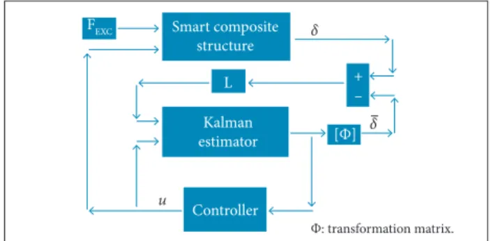
Active modal control is used as control strategy for a smart composite structure as shown in Fig. 1. In this strategy, δ is the displacement, X stands the modal states, FEXCis the external forces and u is the control efort.
where:
x(t): derivative of x(t) with respect to time; x(t): state vector;
[A]: n x n dynamic matrix; [B]: n x m input matrix; [C]: s x n output matrix; {u(t)}: input force; {y(t)}: output vector; n: order of the system; m: number of inputs; s: number of outputs.
he system is called balanced if the solutions to the following Lyapunov equations (Eq. 14 and Eq. 15) are P = Q = diag (σ1, σ2,…, σn):
Figure 1. Active modal control based on modal state feedback control (adapted from Koroishi et al., 2014).
.
.
where:
[P] and [Q]: respectively, the controllability and observability Gramians;
σi (i = 1, 2, ..., n): the singular values of the system (σ1 ≥ σ2 ≥ … ≥ σn ≥ 0).
Every σi is associated with a state xi of the balanced system. Its value quantifies the contribution that xi makes to the input-output behavior of the system. As σ1 ≥ σ2,then x1 affects the behavior of the system more than x2, due to the fact that the singular values are ranked from the most important to the least important one. In the balanced realization, the fidelity of the reduced model with respect to the full model (A, B, C) depends on the relation σr ≥ σr+1, where r is the reduced model order. Thus, the reduced state space system is given by:
In the strategy shown in Fig. 1, the smart composite structure represented by Eq. 11 was written in the state space form as represented by Eqs. 12 and 13 for the simulations.
The advantage of using active modal control is that this technique is very effective for flexible structures applications, requiring a reduced number of actuators and sensors.The states are then used by the controllers to determine the control force.
The estimator is responsible for determining the modal states required by the controllers. The Kalman estimator is able to estimate the states by using noise contaminated measurement signals. More details regarding the Kalman estimator can be found in the literature (Welch and Bishop, {x(t)} = [A]{x(t)} + [B]{u(t)}
{y(t)} = [C]{x(t)}
[A][P] + [P][A]T + [B][B]T = 0
[A]T [Q] + [Q][A] + [C]T [C] = 0
{xr(t)} = [Ar]{xr(t)} + [Br]{ur(t)}
{yr(t)} = [Cr]{xr(t)}
(12)
(13)
(14)
(15)
(16)
(17)
.
Smart composite structure
Kalman estimator
Controller FEXC
L
u
δ
δ + –
[Φ]
1995; Anderson and Moore, 1979; Durbin and Koopman, 2002). The Kalman estimator is represented by Eq. 18:
[Rlqr]: positive deined hermitian matrix or real symmetric that weights the energy cost of each controller (Simões, 2006).
By substituting Eq. 19 into Eq. 20, it is also possible to obtain the controller gain [K].
LINEAR MATRIX INEQUALITIES
LMI is a powerful tool used in many mathematical problems. hey were irst presented by Aleksandr Mikhailovich Lyapunov, thus forming the well-known Lyapunov heory (Boyd et al., 1994). He demonstrated that the diferential equation:
is stable (all trajectories converge to zero), if and only if there is a positive-deinite matrix Plmisuch that:
where:
[L]: gain matrix. his matrix was determined by using the command lqe.m in the sotware Matlab®;
δ(t): displacement vector;
δ(t): estimated displacement vector.
Figure 1 shows that, in the modal state feedback control, a number of controllers are necessary. he method requires the modal displacements and modal velocities to determine the control efort of the controllers. For this purpose, the Linear Quadratic Regulator, solved by LMI, was used to determine the gains of the controllers. his method permits to take into account slight nonlinearities and uncertainties in the model.
LINEAR QUADRATIC REGULATOR
LQR has a very important role in the design of multivariable control of dynamic systems, not only as a powerful control technique, but also because it represents the source of many recently developed procedures for designing linear MIMO systems. Besides providing a methodology to control the feedback gain, the linear quadratic regulator ensures good stability margins for the closed loop system.
he optimal control, i.e. the linear quadratic regulator in the context of the present contribution, is designed, so that the minimization of the performance index leads to the optimization of pre-deined physical quantities (Ogata, 2003). Considering the feedback control given by:
the gain [K] can be determined by the minimization of the performance index given by Eq. 20.
where:
[Qlqr]: positive deined hermitian matrix (positive deinite or semi-deinite) or real symmetric that weights each state;
he inequality given by Eq. 22 is known as the Lyapunov inequality.
he advantage of using LMI for determining the controller gain is the possibility of assuming that the parameters of the model involve uncertainties.
Currently, LMI have been the object of study by many researchers around the world, aiming at diferent applications, such as: control of continuous and discrete systems in time domain, optimal and robust control (Van Antwerp and Braatz, 2000; Silva et al., 2004), model reductions (Assunção, 2000), control of non-linear systems, theory of robust ilters (Palhares, 1998), besides detection, location and quantiication of faults (Abdalla et al., 2000; Wang et al., 2007).
LINEAR QUADRATIC REGULATOR USING LINEAR MATRIX INEQUALITIES
Several authors have considered applications of LQR; however, not so many have discussed the LMI version of this controller (Johnson and Erkus, 2002). A version of LQR solved by LMI is illustrated in Erkus and Lee (2004). The authors of this contribution show that the problem LQR-LMI is described by:
{x
.
r(t)} = [Ar[{xr(t)} + [Br]{u(t)} + [L]{δ(t)-δ(t)}.
(18)
(19)
(20)
(23) {u(t)} = -[K]{x(t)}
(21)
(22) [A]T[P
lmi] + [Plmi][A] > 0 {x(t)} = [A]{x(t)}
min tr([Qlqr][Plmi]) + tr([Xlmi]) +
tr([Ylmi]N) }+ tr ([N]TY lmi
T)
subjected to:
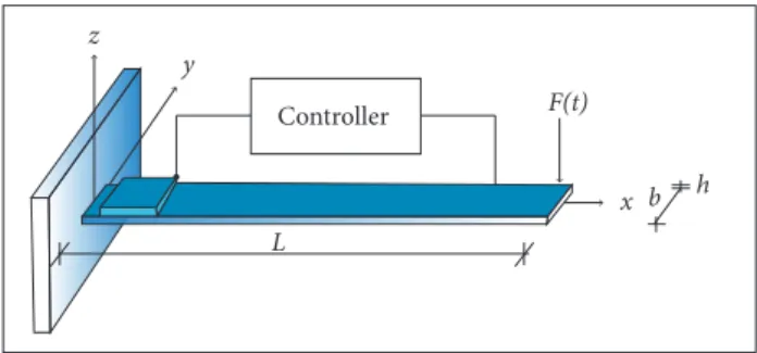
A piezoelectric ceramic actuator of dimensions 45.9 x 25.5 mm2 is bonded to the beam’s top surface, 1 mm away from the clamp. he composite laminate has a total of 5 layers made of graphite/ epoxy and oriented as: 45°/0°/45°/0°/45°. he layers oriented at 0° are parallel to the x axis. he thicknesses of the layers are 0.2 mm and the thickness of the piezoceramic actuator is 1 mm.
The constants of elastic stiffness of the beam made of AS4/3501 carbon/epoxy composite are (given in GPa): C11 = 173.6; C22 = C33 = 7.61; C12 = C13 = 2.48; C23 = 2.31; C44= 1.38; C55 = C66 = 3.45. he PZTs are: C11 = C22 = C33 = 102.23; C12 = C13 = C23 = 5.035; C44 = C55 = C66 = 2.594. he PZT patch piezoelectric constants are (given in C/m2): e
31 = -18.300; e32 = e33 = -9.013. he electric permissivities are (given in F/m): χ11 = χ22= χ33 = 1800ε0 . he mass densities, in kg/m3, are 1,578 for the composite laminated material and 7,700 for the PZT patch. he FE model has been derived by using a 10 x 1 uniform mesh. he excitation force (1 N) was applied at point II and the time domain structure responses were captured at point I (see Fig. 2). he piezoelectric actuator is connected to an active control system, and the vibration amplitudes are to be minimized over time. To proceed as similar as possible to experimentation condition, band-limited white noise is superposed to the calculated displacements.
hree cases of active vibration control were analyzed: a Comparison between the controllers designed using Eqs. 18
and 19 and the robust controllers designed using Eqs. 22, 23 and 24. In this case, there is no uncertainty in the models, thus forming the deterministic case.
b Robustness analyses considering variation in the model of smart composite structure so that the uncertainties were considered in the dynamical matrix [A] + [ΔA]. c Robustness analyses considering variation in the dynamical matrix of Kalman Estimator [Ar] + [ΔAr]. The variation applied in case (b) corresponds to possible modiications in the structure, and the variation where:
N: noise position vector; [Xlmi] and [Ylmi]: LMI solutions; tr( ): denotes the matrix trace; Bw: disturbance matrix.
Equation 23 was adapted from the minimization of the performance index given by Eq. 20. hen, the inluence of noise was incorporated in the process of performance index minimization. By solving Eq. 23 with the constraints considered in Eq. 24, the controller gain is:
DESIGN OF ROBUST CONTROLLERS USING LMI he major advantage of LMI design is to enable speciications such as stability degree requirements, decay rate, input limitation for the actuators and output peak bounder. It is also possible to assume that the model’s parameters involve uncertainties (Ogata, 2003). he LMI is a very useful tool for problems with constraints where the parameters vary according to a range of values. The design of robust controllers used in this contribution was previously presented by Assunção and Teixeira (2001). A system with politopic uncertainties is stable if there is [X] and [G] such as the following LMI are feasible:
where:
Figure 2. Composite cantilever beam with active vibration control. [A][P] - [B][Ylmi] + [P][A]T - [Y
lmi]
T[B]T + [B w][Bw]
T < 0
[G] = [Ylmi] [Plmi]-1 [Xlmi] [Ylmi]T
[Ylmi] [Plmi]
> 0 [Rlqr]1/2
[Rlqr]1/2
(24)
(25)
(26)
i = 1, 2, …, m (m is the number of uncertainties); [X]: LMI solution.
Equation 23 was used for the robust control using LQR, and the constraints (Eq. 24) were arranged in the form given by Eq. 26.
NUMERICAL SIMULATIONS
he studied laminated composite beam, illustrated in Fig. 2, has 306 mm length (L), 25.5 mm width (b) and 1 mm thickness (h).
[Ai][X] Bi][G] + [X][Ai]T - [G]T[B i]
T < 0
[X] > 0
Controller
L y z
h b F(t)
x
.
.
considered in case (c) corresponds to uncertainties in terms of system identiication. In both cases, (b) and (c), only non-parametric uncertainties were considered, and the level of these uncertainties was 10% around the nominal value. he samples of the uncertainty term Δ are determined by using Monte Carlo simulation associated with latin hypercube. he number of samples was 100.
For the irst two modes, the system was observable and controllable. For these two modes, four uncertain modes result. Table 1 presents the four uncertain model conigura-tions (matrix Ai). hese models were used to determine the robust controllers.
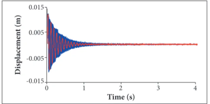
Figure 6. Impact response (case b): deterministic value (red line) and envelope (blue lines).
Figure 3. Impact response.
Figure 5. Control effort.
Figure 4. Frequency response function.
NUMERICAL RESULTS
Figures 3, 4 and 5 present, respectively, the impact response, the frequency response function (FRF), and the control efort for case (a).
By analyzing these results, it is possible to observe that the system was controlled using the conventional controllers and robust controllers. he results were very similar for both controllers. he amplitude attenuation is obtained for a time smaller than 1 s (see Fig. 5).
he FRF is presented in Fig. 4. he irst two modes were attenuated (almost 16.70 dB for the irst frequency and 11.65 dB for the second frequency). Besides, no spillover efects are observed for higher modes (see Fig. 10b).
Ai Mode 1 Mode 2
-10% +10% -10% +10%
1 X -- X
--2 X -- -- X
3 -- X X
--4 -- X -- X
Table 1. Uncertain model (matrix Ai).
Figures 6 to 11 present results for case (b). hese results are divided in two groups, namely conventional controllers (Figs. 6, 7 and 8) and robust controllers (Figs. 9, 10 and 11).
Figure 7. Frequency response function (case b): deterministic value (red line) and envelope (blue lines).
Time (s)
Control – off
Control – on Robust control - on
Dis
p
lac
eme
n
t (m)
-0.015
0 1 2 3 4
-0.005 0.005 0.015
Frequency (Hz)
Control – off
Control – on Robust control - on
20* l
o
g (δ/
FE
XC
) (dB)
0 100 200 300 400 500
-100 -50 0
Time (s)
Control – on Robust control - on
V
o
ltage (V
)
0 1 2 3 4
-0.02 0.02
0
Time (s)
Dis
p
lac
eme
n
t (m)
0 1 2 3 4
-0.015 0.015
0.005
-0.005
Frequency (Hz)
20* l
o
g (δ/
FE
XC
) (dB)
0 100 200 300 400 500
In terms of impact response, Figs. 6 and 9 demonstrate that the use of robust controllers results in an envelope slightly smaller than the one obtained using conventional controllers. he same trend is observed in the control efort presented by Figs. 8 and 11. he disadvantage of using robust controllers is observed in terms of energy consumption since the control efort required when using robust controllers is bigger than the one associated with conventional controllers.
In case (b) (which considers uncertainties in the dynamical matrix of the smart composite structure), better results in terms of vibration attenuation were found (using robust controllers when the system presents variation in the model). However, these controllers lead to higher energy consumption.
Figures 12 to 17 present results for case (c), which considers uncertainty in the dynamical matrix used by the Kalman estimator. hese results are divided in two groups: conventional controllers (Figs. 12, 13 and 14) and robust controllers (Figs. 15, 16 and 17). he irst aspect to point out in the results obtained for case (c) is that they present envelopes smaller than those associated with case (b) — when variation is considered in the structure’s model, the natural frequency varies according to this variation, once the dynamic matrix changes with the value of Δ. he same Figure 8. Control effort (case b): deterministic value (red line)
and envelope (blue lines).
Figure 9. Impact response (case b) - robust control: deterministic value (red line) and envelope (blue lines).
Figure 10. Frequency response function (case b) - robust control: deterministic value (red line) and envelope (blue lines).
Figure 11. Control effort (case b) - robust control: deterministic value (red line) and envelope (blue lines).
Figure 13. Frequency response function (case c): deterministic value (red line) and envelope (blue lines). Figure 12. Impact response (case c): deterministic value (red line) and envelope (blue lines).
Time (s)
V
o
ltage (V
)
0 1 2 3 4
-0.02 0.02
0
Time (s)
Dis
p
lac
eme
n
t (m)
0 1 2 3 4
-0.015 0.015
0.005
-0.005
Frequency (Hz)
20* l
o
g (δ/
FE
XC
) (dB)
0 100 200 300 400 500
-150 -50 50
Time (s)
V
o
ltage (V
)
0 1 2 3 4
-0.02 0.02
0
Time (s)
Dis
p
lac
eme
n
t (m)
0 1 2 3 4
-0.015 0.015
0.005
-0.005
Frequency (Hz)
20* l
o
g (δ/
FE
XC
) (dB)
0 100 200 300 400 500
Figure 17. Control effort (case c) - robust control: deterministic value (red line) and envelope (blue lines).
Figure 20. Difference between maximum and minimum voltage. Figure 16. Frequency response function (case c) - robust
control: deterministic value (red line) and envelope (blue lines).
Figure 19. Difference between maximum and minimum FRF. Figure 15. Impact response (case c) - robust control:
deterministic value (red line) and envelope (blue lines).
Figure 18. Difference between maximum and minimum displacement.
trends are not observable in case (c), because, in this case, the variation is applied in the dynamic matrix of the estimator.
Based on the inluence of the variation applied in the dynamic matrix of the estimator, it is possible to observe better results in terms of vibration attenuation when using robust controllers. Figure 15 shows that the use of robust controllers lead to a better controlled response as compared with the determinist response. However, the energy consumption increases in the irst oscillations that result from the impact response (please compare Fig. 17 with Fig. 14).
A comparison between the results obtained for cases (b) and (c) was performed. his comparison was based on the
diference between the maximum and the minimum value of each envelope. Figures 18, 19 and 20 present, respectively, the interval of the controlled response, FRF, and control efort.
Figure 14. Control effort (case c): deterministic value (red line) and envelope (blue lines).
Time (s)
V
o
ltage (V
)
0 1 2 3 4
-0.04 0.04
0
Time (s)
Dis
p
lac
eme
n
t (m)
0 1 2 3 4
-0.015 0.015
0.005
-0.005
Frequency (Hz)
20* l
o
g (δ/
FE
XC
) (dB)
0 100 200 300 400 500
-100 -20
-60 20
Time (s)
V
o
ltage (V
)
0 1 2 3 4
-0.1 0.1
0
Time (s)
Stochastic model – control – on Stochastic model – robust control – on Stochastic estimator – control – on Stochastic estimator – robust control – on
∆(δ) (m)
0 1 2 3 4
0 0.01 0.02
Frequency (Hz)
Stochastic model – control – on Stochastic model – robust control – on Stochastic estimator – control – on Stochastic estimator – robust control – on
∆(20* l
o
g(δ/
FE
XC
)) (dB)
0 200 400
0 40 80
Time (s)
Stochastic model – control – on Stochastic model – robust control – on Stochastic estimator – control – on Stochastic estimator – robust control – on
∆(V
o
ltage) (V
)
0 1 2 3 4
CONCLUSIONS
he present contribution was dedicated to the design of robust controllers using LQR solved by LMI. he motivation for this research effort is that LMI approach represents a powerful mathematical tool that exhibits relevant characteristics which facilitate the resolution of control problems involving uncertainties. his coniguration corresponds to real world applications, particularly in the case of aerospace structure design.
For illustration purposes, the present study aimed at applying the LMI technique to beams made of composite material. A model reduction method associated with the balanced realization technique was performed.
he results have revealed that the number of considered modes (two) was suicient to achieve satisfactory control. It should be emphasized the importance of balanced realization on this stage, since this technique ranks the modes in order of relevance, regarding the dynamic behavior of the system. his means that the considered modes are the most important to the system response.
Also, with respect to the modes, the robust controller technique was efective on the irst two modes and no spillover efects were observed in the higher modes. he results demonstrated
the efectiveness of the methodology proposed, based on the comparison of the controlled and uncontrolled system responses. he presented results demonstrate the great potential of the proposed methodology (using LMI), since it led to very similar results as compared with those obtained via LQR solved by classical Ricatti equations. hese trends were clearly observed in case (a). Cases (b) and (c), which consider variation in the dynamic matrix of the smart composite structure and Kalman estimator, respectively, demonstrated better results in terms of vibration attenuation using robust controllers (when the system presents variation in the model). However, the robust controllers require bigger energy consumption than the conventional ones.
ACKNOWLEDGEMENTS
he authors are thankful to the Brazilian Research Agencies Fundação de Amparo à Pesquisa do Estado de Minas Gerais (FAPEMIG), Conselho Nacional de Desenvolvimento Cientíico e Tecnológico (CNPq) and Coordenação de Aperfeiçoamento de Pessoal de Nível Superior (CAPES) for the inancial support to this work through the INCT-EIE.
REFERENCES
Abdalla, M.O., Zimmerman, D.C. and Grigoriadis, K.M., 2000, “Reduced Optimal Parameter Update in Structural Systems Using LMIs”, Proceedings of the 2000 American Control Conference, Chicago, USA.
Anderson, B.D.O. and Moore, J.B., 1979, “Optimal Filtering”, Prentice-Hall, New Jersey, USA, 357p.
Assunção, E., 2000, “Redução H2 e H∞ de Modelos através de Desigualdades Matriciais Lineares: Otimização Local e Global”, Ph.D. Thesis, Universidade Estadual de Campinas, Campinas, Brazil.
Assunção, E. and Hemerly, E.M., 1992, “Redução de Modelos de Sistemas Dinâmicos”, Proceedings of the 9º Congresso Brasileiro de Automática, Vol. 1, Vitória, Brasil.
Assunção, E. and Teixeira, M., 2001, “Projeto de Sistema de Controle Via LMIs usando o MATLAB”, Escola Brasileira de Aplicações em Dinâmica e Controle - APLICON-USP, São Carlos, Brazil.
Boyd, S., Balakrishnan, V., Feron, E. and El Ghaoui, L., 1994, “Linear Matrix Inequalities in Systems and Control Theory”, Retrieved in September 06, 2015, from http://www.web.stanford.edu/~boyd/ lmibook/lmibook.pdf
Cen, S., Soh, A., Long, Y., Yao, Z., 2002, “A New 4-Node Quadrilateral FE Model with Variable Electrical Degrees of Freedom for
the Analysis of Piezoelectric Laminated Composite Plates”, Composite Structures, Vol. 58, No. 4, pp. 583-599. doi: 10.1016/S0263-8223(02)00167-8
Chee, C.Y.K., 2000, “Static Shape Control of Laminated Composite Plate Smart Structure Using Piezoelectric Actuators”, Ph.D. Thesis, University of Sydney, Sydney, Australia.
Chee, C.Y.K., Tong L. and Steven, G., 2000, “A Mixed Model for Adaptive Composite Plates with Piezoelectric for Anisotropic Actuation”, Computers & Structures, Vol. 77, No. 3, pp. 253-268. doi: 10.1016/S0045-7949(99)00225-4
Conceição, S.M., Bueno, B.N., Cavalini Jr, A.A., Abreu, G.L., Melo, G.P. and Lopes Jr, V., 2009, “Model Reduction Methods for Smart Truss like Structure”, Proceedings of 8th Brazilian Conference on Dynamics, Control and Applications, Bauru, Brasil.
Durbin, J. and Koopman, S.J., 2002, “Time Series Analysis by State Space Methods”, Oxford University Press, Oxford, UK.
Erkus, B. and Lee, Y.J., 2004, “Linear Matrix Inequalities and Matlab LMI Toolbox”, University of Southern California Group Meeting Report, Los Angeles, USA.
“Numerical and Experimental Modal Control of Flexible Rotor Using Electromagnetic Actuator, Mathematical Problems in Engineering, Vol. 2014, No. 2014, pp. 1-14. doi: 10.1155/2014/361418
Laub, A.J., Heath, M.T., Paige, C.C. and Ward, R.C., 1987, “Computation of Systems Balancing Transformation and Other Applications of Simultaneous Diagonalization Algorithms”, IEEE Transactions on Automatic Control, Vol. 32, No. 2, pp. 115-122. doi: 10.1109/TAC.1987.1104549
Lima, A.M.G., Faria, A.W. and Rade, D.A., 2010, “Sensitivity Analysis of Frequency Response Functions of Composite Sandwich Plates Containing Viscoelastic Layers”, Composites Structures, Vol. 92, No. 2, pp. 364-376. doi: 10.1016/j.compstruct.2009.08.017
Ogata, K., 2003, “Engenharia de Controle Moderno”, Prentice-Hall do Brasil, São Paulo, Brazil, 788p.
Palhares, R.M., 1998, “Filtragem Robusta: uma Abordagem por Desigualdades Matriciais Lineares”, Ph.D. Thesis, Universidade Estadual de Campinas, Campinas, Brazil.
Reddy, J.N., 1997, “Mechanics of Laminated Composite Plates: Theory and Analysis”, Second Edition, CRC Press, London, UK.
Saravanos, D.A., Heyliger P.R. and Hopkins D.A., 1997, “Layerwise Mechanics and Finite Element for the Dynamic Analysis of Piezoelectric Composite Plates”, International Journal of Solids and
7683(96)00012-1
Silva, S., Lopes Jr, V. and Assunção, E., 2004, “Robust Control to Parametric Uncertainties in Smart Structures Using Linear Matrix Inequalities”, Journal of the Brazilian Society of Mechanical Sciences and Engineering, Vol. 26, No. 4, pp. 430-437. doi: 10.1590/S1678-58782004000400008
Simões, R.C., 2006, “Controle Modal Ótimo de um Rotor Flexível Utilizando Atuadores Piezelétricos do Tipo Pilha”, Ph.D., Universidade Federal de Uberlândia, Uberlândia, Brazil, 133p.
Thinh, T.I. and Ngoc, L.K., 2010, “Static Behavior and Vibration Control of Piezoelectric Cantilever Composite Plates and Comparison with Experiments”, Computational Materials Science, Vol. 49, No. 4, S276-S280. doi: 10.1016/j.commatsci.2010.03.016
Van Antwerp, J.G. and Braatz, R.D., 2000, “A Tutorial on Linear and Bilinear Matrix Inequalities”, Journal of Process Control, Vol. 10, No. 4, pp. 363-385. doi: 10.1016/S0959-1524(99)00056-6
Wang., H.B., Wang, J.L. and Lam, J., 2007, “Robust Fault Detection Observer Design: Iterative LMI Approaches”, Journal of Dynamic Systems, Measurement, and Control, Vol. 129, No. 1, pp. 77-82. doi: 10.1115/1.2397155