ABSTRACT: As the representative of manufacturing industry, aircraft assembly lacks of effective method to forecast man-hour. The forecasting accuracy of existing methods is universally pretty low. On the basis of full analysis of aircraft assembly’s feature, this study proposes a forecasting model based on support vector machine (SVM), which is optimized by particle swarm optimization. It can carry out quantitative prediction of the process’ man-hour during aircraft’s assembly. Firstly, we decompose aircraft’s assembly work by the concept of work breakdown structure. Further, the process parameters related to man-hour were listed and we made necessary correlation analysis of these historical data. Parameters with high contribution are then used as input of forecasting model. A new forecasting model utilizing SVM is proposed, which carries out the process as the minimum research granularity. Its performance is compared with back propagation neural network. The process of automatic drilling & riveting is adopted as an example in order to present and validate the model. Experimental results relect that SVM has high forecast precision and good itness, so that it is suitable for small sample prediction. Through the optimization, it can effectively predict man-hour of assembly work in a short time while maintaining suficient accuracy.
KEYWORDS: SVM, PSO, Aircraft assembly, Man-hour prediction, Predictive model.
The Prediction of the Man-Hour in Aircraft
Assembly Based on Support Vector Machine
Particle Swarm Optimization
Tingting Yu1, Hongxia Cai1
INTRODUCTION
Due to the large size, complex shape and numerous parts, the amount of aircraft assembly accounts for more than a half of total aircrat manufacturing (Enming, 2005). Aircrat assembly is the process of assembling a large number of aircrat parts according to a certain order and gradually putting them into components, forge pieces and sub-units. Finally, the components are butted into an entire aircrat. herefore, aircrat assembly, as a very important part in the industry of large passenger aircrat, need be carried out strictly in accordance with the production plan, which includes not only the distribution of production site, equipment and resources, but also the arrangement of man-hour. Man-hour quota not only directly afects the working time, the utilization rate of the equipment, but also is the basic unit for calculating cost (Bin and Zuhua, 2006). At the same time, it is widely used as a toll for cost management in manufacturing enterprises. herefore, man-hour prediction as the core of man-hour quota management is directly related to economic accounting, production schedule control, resource optimization, production cycles shortening, cost control and product quotation. Besides, it ultimately promotes the improvement of labor productivity of enterprises and enhances their market competitiveness (Chao and Danchen, 2010).
Just realizing this point, advanced international aircraft manufacturing companies have changed the condition that arranges production plan passively into predicting man-hours actively. hrough the analysis, they can determine the production planning and production scheduling. Since the civil aircrat industry in China started late, there is a big gap in man-hour
1.Shanghai University – Shanghai – China.
Author for correspondence: Hongxia Cai | Shanghai Key Laboratory of Intelligent Manufacturing and Robotics | Shanghai University | Yanchang Road 149, Zhabei District | 200072 – Shanghai – China | Email: [email protected]
prediction between China and international level. he overall utilization of workshop equipment is less than 40% (Changqing et al., 2011). At present, man-hour prediction approach is mainly estimated through workers’ experience, analogy and other methods based on relevant technical iles and it has to calculate the production hours according to the detailed production process step by step. his method has the disadvantages of slow speed, low eiciency, big error and high dependence on personal experience, which causes the uncertainties in production planning and scheduling (Yajie et al., 2013). As a result, it is unable to adapt to the needs of modernization, scientiic and ine production management, seriously afecting the production schedule and production eiciency.
Diferent industries including computer, ships, computer numerical control (CNC) machining and aerospace have devoted a lot to develop a series of man-hour management sotware with good performance. Man-hour prediction has been treated as an important method to improve production eiciency, optimize resource management and shorten the manufacturing cycle. Among this series, the most representative are Timesheet, AceTeamwork, Appfarm, G TimeSheet and Replicon Web TimeSheet. However, most of these programs are integrated with enterprise resource planning (ERP) system, manufacturing execution system (MES) and computer aided process planning (CAPP). heir core function is to manage and share the document and the information during production. hereby, man-hour management is deicient. So far, the time forecasting methods in manufacturing industry mainly includes standard data method, simulation method by numerical control (NC) program and artiicial intelligence method. Boothroyd (1994) used an injection molding as standard and estimated other injection moldings rely on the relative value. Wang et al. (2002) used a triangular fuzzy number to estimate ready time and solved the ready time scheduling problem. Siller (2006) predicted the man-hour by simulation on NC program and specially forecasted the cycle of high-speed milling. Coelho (2010) also presented a practical mechanistic method for milling time estimation when machining free-form geometries by process simulation method. Bustillo and Correa (2012) presented a predictive model by using artiicial intelligence to optimize deep drilling operations under high speed conditions for the manufacture of steel components. A feed-forward neural network and support vector machine (SVM) are used for surface’s roughness prediction by Çaydaş and Ekici (2012). Two sot computing techniques, namely, neuro
fuzzy logic technique and support vector regression technique were used for the assessment of the remaining useful life (RUL) of cutting tools (Gokulachandran and Mohandas, 2013). Li et al. (2012) tested various possible linear regression methods by using six dependent variables to enhance the production yield in the color ilter (CF) manufacturing process. In his study, the Support Vector Machine for Regression (SVR) model was found to be the most appropriate for forecasting manufacturing performance. In these methods, SVM owns few adjustable parameters, quick computing speed, accurate rate, good robustness and good generalization ability (Cao and Tay, 2003). In the absence of more background information, it can also achieve high prediction accuracy (Kotsiantis, 2007). It solves the non-linear, high-dimension and local minima and some other issues efectively.
On the basis of extensive study of time prediction methods and the present situation in manufacturing industry, aircraft assembly work is broken down according to the concept of work breakdown structure (WBS). Then, we listed various related process parameters. Using process as the smallest granularity, the predictive model based on SVM is established. Typically, one of the important processes — automatic drilling & riveting process — is introduced as an example to verify the model. More-over, the predictive performance is also compared with the back propagation (BP) neural network. Eventually, considering that the grid algorithm is time-consuming, we choose to use PSO algorithm and genetic algorithm (GA) to optimize the predictive model.
PROBLEM AND ALGORITHM
DESCRIPTION
f(x) = ωφ(x) + b
f(x) = Σk
i=1(αi - α
*
i) ϕ(xi) ϕ(x) + b =
Σk
i=1(αi - α
*
i) K(xi - xj) + b
(1)
(4) man-hour data and is the foundation for time management and
prediction, the minimum unit of our research is the process. A complex project can be decomposed into a series of clearly detailed subprojects by WBS, which groups project elements through deliverables-oriented ideas. hese elements organize and deine the work scope of a whole project. he subprojects decomposed by WBS cover labor and non-labor resources, including man-hour information which provide an important foundation for schedule planning, resource requirements, cost budget, purchasing plan etc. Top-down approach is applied in this paper to complete the WBS decomposition. Namely, aircrat assembly is decomposed by the order of project-sortie-workstation-station-process. hen, we can predict the man-hour of each process. he total time of a project can be obtained by accumulating all the process’ man-hour.
SUPPORT VECTOR MACHINES
SVM is established on the basis of statistical learning theory (Cristianini and Shawe-Taylor, 2000). It is a kind of machine learning method which applies the principle of Vapnik-Chervonenkis (VC) dimension and structural risk minimization. It extensively overcomes the problems of “dimension disaster” and “too much learning” that exist in traditional machine learning methods such as neural network (Peng and Wang, 2009; Choi, 2009). It shows a lot of unique advantages in solving small sample, non-linear and high dimensional recognition problems. Especially, it is widely used in pattern recognition, regression analysis, function estimation, time series forecasting and other ields (Ge et al., 2004; Guo and Li, 2003).
We establish a training set containing n training sam-ples as {(xi, yi), i = 1, 2, ..., n}. Among them, xi (xi Є Rd) is the ith input column vector of training samples. In this study, they are a series of variables associated with the man-hour; xi = [xi1, x
i 2,..., x
i d]т, y
i Є R , is the corresponding output value, namely, process’ hour, and d is the number of rows. It is clear that man-hour forecasting belongs to the typical non-linear problem. he regression function in high dimensional space, which represents the relationship between process’ man-hour and input variables, can be expressed as:
ζ limits the error of the regression function and slack variables, , ( ≥ 0, ≥ 0)are introduced. Namely,
where C is the penalty factor.
In order to simplify the learning process of SVM, the problem can be changed as follows by using Lagrange function:
(2)
(3)
where K(xi,xj) = ϕ(xi) ϕ(xj) (the inner product of xi and xj) is kernel function.
We applied radial basis function (RBF) kernel function K(x,y) = exp ( ) in our study. Assuming that the optimal solution of Eq. 3 is , α = [α1, α2, ..., αk], α* = [α*
1, α *
2, ..., α *
k], then we get the regression function:
y x
σ2 2
In SVM regression problems, the parameter σ controls the lexibility of RBF kernel function. It directly afects the generalization performance of models. he penalty factor C plays the role of balancing decision function and error classiication samples, which inluences the generalization ability of the model.
PARTICLE SWARM OPTIMIZATION
Particle swarm optimization (PSO) was irstly proposed Kennedy and Eberhart (1995) and it is based on the research of group behavior of birds. PSO looks each individual in n-dimension as a particle without weight and volume. It lies in the search space with a certain speed. he light speed is adjusted dynamically by individual light experience and group lying experience.
In a n-dimensional space, the ith particle’s position and speed can be expressed respectively as: X1 = (Xi1, Xi2, ..., Xin), Vi = (Vi1, Vi2, ..., Vin). he optimal position that each particle has experienced is Pi = (Pi1, Pi2, ..., Pin). he global optimal position where φ(x) represents the high dimensional feature space.
Pg(t)Є{P0(t), ... Pg(t)}| f
(
Pg(t))
min{f(
P0(t))
, ... f(Ps(t))
}Vi(t+1) = wVi(t)+ c1r1(Pi(t)- xi(t)+ c2r2
(
Pg(t) - Xi(t))
Xi(t+1) = Xi(t)+ Vi(t+1)
(5)
(6)
(7)
is Pgbest = (Pg1, Pg2, ..., Pgn). Pg(t) means the best location of a
population containing s particles.
and some other kind of parameters. Besides, the relationship among these factors is complex, leading the forecasting work to a typical non-linear problem. As input parameters of the predictive model, man-hour driving factors directly affect the predictive accuracy of the model. So, we need to analyze this inluence from aspects of the contribution and relevance of the factors. his step is to make correlation analysis of related factors by using statistical product and service solutions (SPSS), an IBM sotware widely used in statistical analysis, data mining, prediction analysis and decision support.
Sample data acquisition and processing
he data’s changing scope of sample set imposes an important inluence on training model. he sample set should relect the characteristics of a process as far as possible. hen the data were observed and collected, and invalid data were excluded. Due to the big diferences in magnitude and unit, the data should be normalized before establishing the regression model.
Model selection and parameter determination
When building SVM, the selection of kernel function is directly related to the performance of the model. We choose to use radial basis function (RBF) which is widely used owning to its best performance. he penalty factor C and the kernel parameter g directly inluence the accuracy of the predictive model. he role of C is to adjust the learning machine’s conidence interval range in a certain data subspace. Kernel parameter g afects the distribution complexity of sample data’s subspace and determines the minimum error (Keerthi and Lin, 2003). In this study, cross validation is irstly adopted to determine the parameters C and g. Subsequently, we apply PSO to make further optimization and we get the best parameter combinations of C and g.
Sample training and model establishment
Generally, for a given time prediction problem, sample data {x1, x2, x3, ..., xr} are usually divided into 2 parts. he front m data is set as the training sample to build predictive model and the latter n-m data is for prediction test. Model building is actually the process of solving regression function (Eq. 2) by SVM with its good performance.
Application and forecast
Put the input data that need to be forecast in accordance with the speciied format. hen, predict them and make error analysis through the predictive model achieved in step “Sample The updating formula of the ith particle’s velocity and
position are:
a) velocity updating formula:
b) position updating formula:
where w is the inertia coeicient whose value is also in the scope of (0,1); c1 is the cognitive coeicient; c2 is the social learning coeicient. he values of c1 and c2are usually in the scope of (1, 2); r1,r2, are the random number in the scope of (0,1).
he parameters C and g should be considered as a particle in space. Under this assumption, the problem of parameter optimization is substantially to ind the global optimal position of all particles. hen, the SVM model can be optimized by utilizing the advantages of fast global optimization possessed by PSO.
THE PREDICTIVE MODEL BASED ON SUPPORT VECTOR MACHINES-PARTICLE SWARM
OPTIMIZATION MODEL CONSTRUCTION
Historical data is a comprehensive relection of the internal mechanism of a system’s changes (Bing, 2014). he number of historical data shows the mechanism of the changes in an extent. Process’ man-hour is an important basis for reasonable plan and arrangement of production. Man-hour related data are dependent on the speciic process. herefore, process is the basic unit for our study. We analyzed the technological characteristics of a speciic process to extract inluence factors. Besides, intrinsic relationships between these factors and the process’ man-hour were further mined through machine learning, so as to achieve the purpose of man-hour prediction.
he steps of establishing the predictive model of SVM are described as follows:
Inluence factors analysis
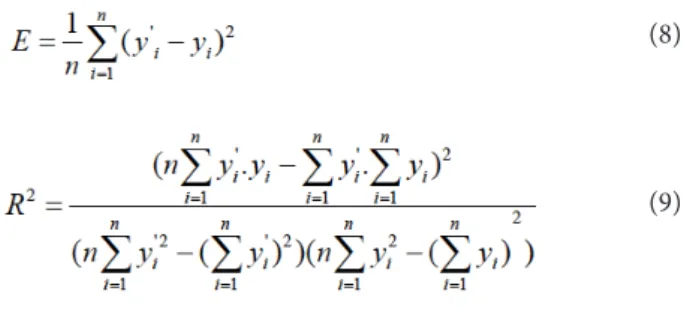
(8)
(9)
Analysis of influence factors Correlation analysis
Randomly distribute the sample set Training set Test set
Comparative analysis
Obtainment of suitable classifier Erros analysis Erros analysis
Train
Best parameter C, g PSO Optimization Determination of initial
velocity and position
Train SVM Establish regression model
Forecast application Real
production
BP model SVM model
Sample collection and processing History
database
Build BP neural network Set parameters
Train network Establish regression model
Train SVM Establish regression model
Select kernel functions Set parameters
IF = f1(Fp,Ft)
T = f(IF,IP,IE,II)
(11) (10)
Figure 1. The man-hour predictive model based on SVM-PSO.
training and model establishment”. For regression problems, the measures to value the performance of a model are mean square error (MSE or E) and determination coeicient (R2):
MAN-HOUR PREDICTION OF AUTOMATIC DRILLING & RIVETING BY SVM-PSO
WBS decomposition demonstrates that the aircrat assembly involves multiple workstations and stations. Assembly work eventually composes a series of assembly process. here is a variety of connections during the course of aircrat assembly, such as riveting, bolting, welding, gluing etc. According to statistics, 70% of the aircrat accidents due to fatigue failure were attributed to the joint connection. Moreover, 80% of the fatigue cracks occurred in hole connection (Liming and Chongneng, 2008). It is visible that connection quality greatly affects the life of an aircraft. Riveting occupies a very important position among different kinds of connections. It is estimated that the amount of assembly labor accounts for about half or even more of the entire aircrat manufacturing labor. And riveting accounts for 30%. Owning to the good fatigue resistance and high reliability, automatic drilling & riveting is widely used in the assembly process of large plane and wing panel. It is an important process for aircrat assembly. herefore, this paper takes automatic drilling & riveting process as an example to conduct the research of man-hour prediction.
ANALYSIS OF THE INFLUENCE FACTORS OF PROCESS’ MAN-HOUR
According to statistics, headless riveting accounts for more than 80% in wing manufacturing process of aircrat ARJ21. Riveting & drilling parameters are the key-factors that afect the eiciency and quality of assembly (Lianxi et al., 2013). Generally, we analyze the driving factors of the automatic drilling & riveting process from the aspects of general features of assembly (IF), processing technic (Ip), equipment parameters (IE) and performance indexes (II). he function relation between man-hour and various factors can be expressed as: where n is the number of test samples; y1(i = 1, 2, …, n) is
the real value of the ithsample; y’
1(i = 1, 2, …, n) is the predictive value of the ithsample. he smaller MSE means the higher prediction accuracy. R2 determines the related degree and the value more closer to 1 indicates the greater itness.
Build the man-hour predictive model based on SVM-PSO as previously mentioned (Fig. 1).
IE = f2(Er, Ec, Ed, Ef, Et, Ep)
T = f(Ft, Er, Ec, Ed, Ef, Et)
Il = fa(Il, IRa,Ih )
T = f(Fp, Ft,Er, Ec, Ed, Ef, Et, Ep, Il, IRa, Ih )
(12)
(15)
(16) (13)
(14)
Fp Ft Er Ec Ed Ef Et Ep Il IRa Ih
Pearson’s
correlation -0.013 0.485 -0.441 -0.468 -0.337 -0.447 0.930 -0.078 -0.209 0.161 0.179
Conspicuousness
(bilateral) 0.927 0.066 0.000 0.000 0.001 0.000 0.001 0.444 0.146 0.265 0.213
Table 1. Correlation comparison of different inluence factors.
y = (ymax - ymin) + (x-xmin)
xmax - xmin + ymin, (ymax = 1, ymin = -1)
The processes can be achieved by automatic drilling & riveting, which mainly includes: drilling, countersinking, glue, nail feeding, fastener installation or completing one or more of these operations. We need to use the combination of these process. So, it is unnecessary to consider process technic when analyzing the inluence factors.
Equipment parameters associated with the man-hour are mainly related to drilling parameters including spindle speed (Er), clamping force (Ec), feed rate (Ed), riveting force (Ef), riveting residence time (Et) and lubrication pressure (Ep). he relation between equipment parameters and man-hour can be expressed as:
we obtained the correlation between each inluence factor and process’ man-hour through various analyses, respectively. Finally, the results are demonstrated in Table 1.
In the mentioned table, Pearson’s correlation coeicient describes the relationship between variables as well as their statistical correlation degree. Pearson’s correlation coeicients bigger than 0.4 mean good correlation, bigger than 0.5 mean strong correlation and bigger than 0.6 represent very strong correlation. Conspicuousness can be understood as probability, which is used to determine the overall conspicuousness diference between reality and hypothesis. It requires conspicuousness levels below 0.05, because 5% can be considered as a small probability event. It is easy to ind from Table 1 that driving factors which inluence the man-hour of automatic drilling & riveting process are:
he indexes of main performance refer to scratch length of hole (Il), surface roughness (IRa) and burr height (Ih).
Ater these considerations, Eq. 10 can be expressed as:
It is found that the major driving factors are extremely related to some other detail parameters. Besides, these parameters may inluence each other or some just have weak inluence. In the current modeling process, we should pay enough attention to the pre-condition that improves the accuracy of the model with least driving factors to reduce the complexity and the noisy interference of the model (Wang et al., 2012).This requires further analysis of the factors’ correlation and contribution. his study used Statistical Package for the Social Sciences (SPSS) to analyze the correlation of 99 sample data extracted from historical database. Firstly, the sample data was saved as in the format ile.sav, which can be recognized by SPSS. hen, the analysis was made to judge the correlation between Fp and process’ man-hour, including Pearson’s correlation and conspicuousness. Similarly,
SAMPLE DATA ACQUISITION AND
PROCESSING
Firstly, we have to screen the sample data extracted from the historical database to eliminate invalid data of unconventional or high reusable degree. hen, 99 valid data were obtained and they were separated into test set (19 data) and training set (80 data) when building the model. he training set and the test set were randomly selected in order to ensure the accuracy of the model. Because the units of Ft,Er, ..., Et are diferent and the magnitude of them difers tremendously, we made the normalization processing of these samples by the following formula:
Ft Er Ec Ed Ef Et T
1 -0.3333 0.1667 -0.1538 -0.1765 -0.2598 0.5 0.2992
2 0.3333 0.8333 0.8462 1 -1 0.5 0.2356
3 -0.3333 0.1667 -0.1538 -0.1765 -0.2598 0.5 0.2992
4 0.3333 0 -0.2308 -0.2941 -0.2598 -0.3 -0.1811
5 0.6667 -0.6667 -0.6154 -0.5882 -0.4173 0.5 0.6252
6 0.3333 -0.5000 -0.6923 -0.2941 -0.5748 1 0.8425
7 -0.6667 0.3333 -0.0769 -0.1765 -0.1024 0.5 0.2402
8 -1 -0.8333 -0.8462 -0.8824 -0.7638 0.5 0.3228
9 -1 0.1667 -0.3846 -0.1765 -0.4173 0.5 0.1811
10 1 0.5000 0.2308 0.2941 0.2126 -1.1102 0.0236
11 -0.5000 0.4167 0.0769 -0.0588 0.1339 -1.1102 -0.1431
12 1 0.5000 0.2308 0.2941 0.2126 -1.1102 0.0236
… … … …
80 -0.3333 0.8333 0.8462 0.8824 0.6850 0.6850 -0.6157
Table 2. Sample set after normalization.
Sample number
P
ro
cess t
ime
20 10 0 1 2 3 4 5 6 7
30 40 50 60 70 80
Comparison of predictive results - SVM(training set)
MSE = 0.00056861 R2 = 0.99682
Real value Predictive value
5 0
2.5 3.5 4.5 5.5 6.5
6
3 4 5
10
Sample number
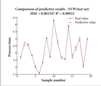
Comparison of predictive results - SVW(test set)
MSE = 0.001547 R2 = 0.98933
P
ro
cess t
ime
15 20
Real value Predictive value
Figure 2. The prediction result of training set. Figure 3. The prediction result of test set.
REGRESSED PREDICTION BASED ON SUPPORT VECTOR MACHINES
We will begin to train the sample data and establish predictive model in this part after completing the mentioned preparations. Firstly, use cross validation (v = 5) to find the best parameters of C and g. Secondly, put the normalized sample data into predictive model and complete sample learning and prediction. The prediction results of training set and test set are shown in Figs. 2 and 3.
Both training set and test set were randomly generated in the experiment, so it could ensure the universality and accuracy of the result. Nevertheless, it is particularly necessary to conduct
comparative analyses on other methods. In order to further validate the performance of the model, we also presented BP neural network to make predict experiment. The forecasting result is shown in Fig. 4.
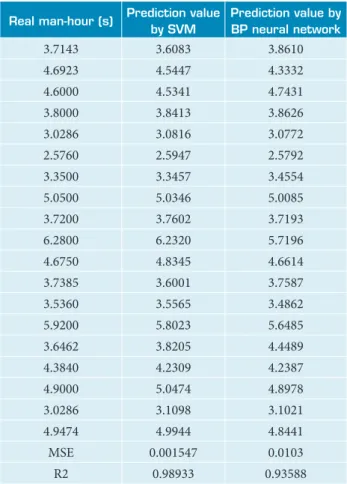
Table 3 assesses the comparison of the forecasting results by SVM and BP neural network.After comparison, it is obvious that the prediction result of SVM is much better than BP neural network. MSE of BP neural network is much higher than SVM and R2 of SVM is closer to 1.
Real man-hour (s) Prediction value by SVM
Prediction value by BP neural network
3.7143 3.6083 3.8610
4.6923 4.5447 4.3332
4.6000 4.5341 4.7431
3.8000 3.8413 3.8626
3.0286 3.0816 3.0772
2.5760 2.5947 2.5792
3.3500 3.3457 3.4554
5.0500 5.0346 5.0085
3.7200 3.7602 3.7193
6.2800 6.2320 5.7196
4.6750 4.8345 4.6614
3.7385 3.6001 3.7587
3.5360 3.5565 3.4862
5.9200 5.8023 5.6485
3.6462 3.8205 4.4489
4.3840 4.2309 4.2387
4.9000 5.0474 4.8978
3.0286 3.1098 3.1021
4.9474 4.9944 4.8441
MSE 0.001547 0.0103
R2 0.98933 0.93588
Table 3. The comparison of the forecasting results.
5 0
2.5 3.5 4.5 5.5 6.5
6
3 4 5
10
Sample number
Comparison of predictive results - BP (test set) MSE = 0.0103 R2 = 0.93588
P
ro
cess t
ime
15 20
Real value Predictive value
Real value Predictive value
The best fitness The average fitness
Sample number
P
ro
cess t
ime
Comparison of predictive results (test set)
MSE = 0.30023075 R2 = 0.98802
Evaluation value
P
ro
cess t
ime
Fitsness curve MSE (PSO method) (c1 = 1.5, c2 = 1.7)
Best c = 0.47548 g = 0.1 CVMSE = 0.80214
0.88
0.86
0.84
0.82
0.8
5.5 6
4.5
3.5
3
0 5 10 15 20
0 50 100 150 200
4 5
2.5 0.9 0.92 0.94
Figure 4. Prediction result of the test set by BP neural network.
Figure 5. The optimization by PSO when maxgen = 200;
pop = 20.
OPTIMIZATION OF MAN-HOUR PREDICTIVE MODEL
The parameters of SVM decide its study performance and generalization ability. In practical application, in order to reduce the dependence of initial sample and improve the accuracy of
SVM model, it is necessary to optimize the parameters of C and g. It means that SVM optimization is actually the optimization of the relevant parameters, namely, quickly ind optimal SVM parameters C and g. Grid search can ind the highest accuracy of classiication, namely, the global optimal solution. However, if you want to ind the best parameters of C and g in greater scope, it will be very time-consuming. With the decrease of the grid density, time grows exponentially. Heuristic algorithm can ind the global optimal solution without traversing all the points in the grid. Currently, the widely used heuristic algorithms for inding optimal parameters are PSO algorithm, genetic algorithm, and simulated annealing algorithm.
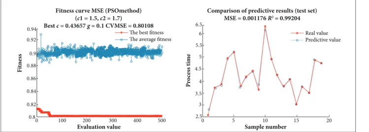
Considering that the principle of PSO and GA is simple and they are easy to implement with high eiciency, this study tried to imply PSO and GA to optimize SVM prediction results obtained above. Figures 5 to 7 show the results of optimization using the PSO and their corresponding prediction results.
The best fitness The average fitness
Real value Predictive value
Sample number
P
ro
cess t
ime
Evaluation value
F
it
ness
Comparison of predictive results (test set)
MSE = 0.001176 R2 = 0.99204
Fitness curve MSE (PSOmethod) (c1 = 1.5, c2 = 1.7)
Best c = 0.43657 g = 0.1 CVMSE = 0.80108
5 0
3 3.5 4 4.5 5 5.5 6 6.5
2.5
10 15 20
0 0.82
0.8 0.84 0.86 0.88 0.92 0.94
0.9
100 200 300 400 500
The best fitness The average fitness
Real value Predictive value
Sample number
P
ro
cess t
ime
Evaluation value
F
it
ness
Comparison of predictive results (test set)
MSE = 0.0019387 R2 = 0.99212
Fitness curve MSE (PSOmethod) (c1 = 1.5, c2 = 1.7)
Best c = 0.43098 g = 0.1 CVMSE = 0.80105
5 0
2 3 3.5 3.4 4.5 5 6 5.5
2.5
10 15 20
0 0.82
0.8 0.84 0.86 0.88 0.9 0.92
100 200 300 400 500
The best fitness The average fitness
Real value Predictive value
Sample number
P
ro
cess t
ime
Evaluation value
F
it
ness
Comparison of predictive results (test set)
MSE = 0.037279 R2 = 0.89392
Fitness curve MSE (GAmethod)
Best c = 0.36324 g = 0.28416 MSE = 0.79735
5 0
1.5 2.5 3 3.5 4 4.5 5.5 5
2
10 15 20
50 0
0.78 0.82
0.8 0.84 0.86 0.88 0.9 0.92 0.94 0.96
100 150 200
Figure 6. The optimization by PSO when maxgen = 500; pop = 50.
Figure 7. The optimization by PSO when maxgen = 500; pop = 100.
The best fitness The average fitness
Evaluation value
F
it
ness
Fitness curve MSE (GAmethod)
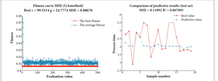
Best c = 99.5514 g = 24.7774 MSE = 0.80678
100 0
0.8 0.82
0.81 0.84
0.83 0.85 0.86 0.87 0.88
200 300 400 500 2.50 5
3.5 4.5 5.5
3 4 5 6
10
Sample number
Comparison of predictive results (test set) MSE = 0.11092 R2 = 0.067095
P
ro
cess t
ime
15 20
Real value Predictive value
The best fitness The average fitness
Real value Predictive value
Sample number
P
ro
cess t
ime
Evaluation value
F
it
ness
Comparison of predictive results (test set)
MSE = 0.39587 R2 = 0.085247
Fitness curve MSE (GAmethod)
Best c = 79.9111 g = 24.2434 MSE = 0.80682
5 0
1 3 4 5 6 8
2
10 15 20
100 0
0.8 0.82
0.81 0.84
0.83 0.85 0.86 0.87 0.88
200 300 400 500
The best fitness The average fitness
Real value Predictive value
Sample number
P
ro
cess t
ime
Evaluation value
F
it
ness
Comparison of predictive results (test set)
MSE = 0.0022812 R2 = 0.98412
Fitness curve MSE (GAmethod)
Best c = 0.43999 g = 1.9551 MSE = 0.82879
5 0
2 3 4 5
2.5 3.5 4.5 5.5
10 15 20
20 0
0.78 0.82
0.8 0.86
0.84 0.88 0.9 0.92 0.94 0.96
40 60 80 100
Figure 9. The optimization by GA when maxgen = 500; pop = 50.
Figure 10. The optimization by GA when maxgen = 500; pop = 100.
The best fitness The average fitness
Real value Predictive value
Sample number
P
ro
cess t
ime
Evaluation value
F
it
ness
Comparison of predictive results (test set)
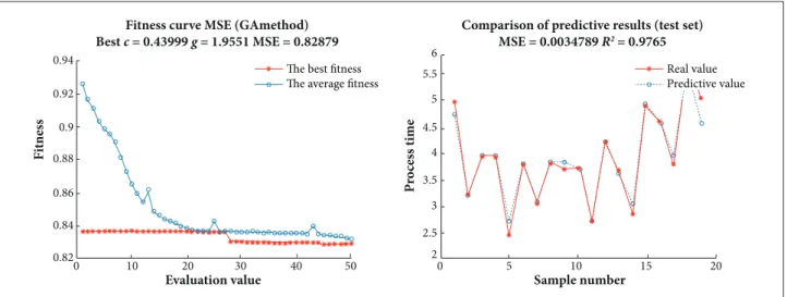
MSE = 0.0034789 R2 = 0.9765
Fitness curve MSE (GAmethod)
Best c = 0.43999 g = 1.9551 MSE = 0.82879
5 0
2 3 4 5 6
2.5 3.5 4.5 5.5
10 15 20
10 0
0.82 0.84 0.86 0.88 0.9 0.92 0.94
20 30 40 50
Figure 12. The optimization by GA when maxgen = 50; pop = 20.
From the optimization experiments of PSO and GA, we could ind that the optimal prediction result is obtained when the maximum number of evolution (maxgen) = 500; population (pop) = 100 of PSO (MSE = 0.0019387; R2 = 0.99212). And
the optimal prediction result is obtained when maxgen = 100; pop = 20 of GA (MSE = 0.0022812; R2 = 0.98412). As a result,
PSO optimization is much better than GA.
CONCLUSION
Aircraft assembly is crucial for its production. It requires effective prediction of man-hour at the beginning of a project, in order to arrange the resources and make production plan reasonably. So far, time prediction mainly relies on work experience. It has a lot of problems, such as slow speed, low efficiency, big error and serious dependence on personal experience. Because the aircraft assembly work is complex and be related to various process’ parameters, this research decomposed the assembly work through the concept of WBS. Then, the parameters that affect process were extracted by analyzing process’ features. Parameters with high correlation are useful. Further, we selected the parameters that highly contributed to predicting man-hour as driving factors. Finally, man-hour predictive model based on SVM was established. Moreover, we made a comparison with BP neural network. As the parameters of C and g extremely determine the model’s performance, this study proposed PSO and GA to optimize the predictive model. Various experiments were
made with different parameters to evaluate MSE and R2.
The results indicate that PSO is more accurate with better fitness. The process of automatic drilling & riveting is used as an example to validate the model with the comparing result of MSE = 0.0019387; R2 = 0.99212. It means that the
MSE between predictive value and the real value is very small and the coeicient of determination reached 0.99212. Namely, the goodness of it is close to 1, which can well relect the relation between the dependent variable (man-hour) and the independent variable (Ft, Er, Ec etc.).
The predictive model based on SVM PSO can effectively forecast the man-hour of different processes according to their driving factors. It is an important approach for enterprises to realize scientific management of the man-hour. In the next step, we will continue to do more studies and experiments so as to make the prediction more precise.
ACKNOWLEDGEMENTS
REFERENCES
Bin, L. and Zuhua, J., 2006, “The Intelligent Man-Hour Estimate Technique of Assembly for Shipbuilding” (In Chinese), Journal of Shanghai Jiaotong University, Vol. 39, No. 12, pp. 1979-1983.
Bing, D., 2014, “Reliability Analysis for Aviation Airline Network Based on Complex Network”, Journal of Aerospace Technology and Management, Vol. 6, No. 2, pp. 193-201. doi: 10.5028/jatm.v6i2.295
Boothroyd, G., 1994, “Product Design for Manufacture and Assembly”, Computer-Aided Design, Vol. 26, No. 7, pp. 505-520.
Bustillo, A. and Correa, M., 2012, “Using artiicial intelligence to predict surface roughness in deep drilling of steel components”, Journal of Intelligent Manufacturing, Vol. 23, No. 5, pp. 1893-1902. doi: 10.1007/s10845-011-0506-8
Cao, L.J., and Tay, F.E.H., 2003, “Support Vector Machine with Adaptive Parameters in Financial Time Series Forecasting”, IEEE Transactions on Neural Networks, Vol. 14, No. 6, pp. 1506-1518. doi: 10.1109/TNN.2003.820556
Çaydaş, U. and Ekici, S., 2012, “Support Vector Machines Models for Surface Roughness Prediction in CNC Turning of AISI 304 Austenitic Stainless Steel”, Journal of Intelligent Manufacturing, Vol. 23, No. 3, pp. 639-650. doi: 10.1007/s10845-010-0415-2
Changqing, L., Yingguang, L., Wei, W. and Yong, L., 2011, “Feature Based Man-Hour Forecasting Model for Aircraft Structure Parts NC Machining”, Computer Integrated Manufacturing Systems, Vol. 17, No. 10, pp. 2156-2162. doi:10.13196/j.cims.2011.10.66.liuzhq.026
Chao, G. and Danchen, Z., 2010, “Man-Hour Quota System Based on Genetic Neural Network” (In Chinese), Computer Applications and Software, Vol. 27, No. 8, pp. 205-208.
Choi, Y.S., 2009, “Least Squares One-Class Support Vector Machine”, Pattern Recognition Letters, Vol. 30, No. 130, pp. 1236-1240.
Coelho, R.T., de Souza, A.F., Roger, A.R., Rigatti, A.M.Y., Ribeiro, A.A.L., 2010, “Mechanistic Approach to Predict Real Machining Time for Milling Free-Form Geometries Applying High Feed Rate”, The International Journal of Advanced Manufacturing Technology, Vol. 46, No. 9-12, pp. 1103-1111. doi: 10.1007/s00170-009-2183-8
Cristianini, N. and Shawe-Taylor, J., 2000, “An Introduction to Support Vector Machines and Other Kernel-Based Learning Methods”, Cambridge University Press, Cambridge, UK. 189p.
Enming, G., 2005, “Flexible Assembly Technology of Foreign Aircraft” (In Chinese), Aeronautical Manufacturing Technology, No. 9, pp. 28-33.
Ge, M., Du, R., Zhang, G. and Xu, Y., 2004, “Fault Diagnosis Using Support Vector Machine with an Application in Sheet Metal Stamping Operations”, Mechanical Systems and Signal Processing, Vol. 18, No. 1, pp. 143-159. doi:10.1016/S0888-3270(03)00071-2
Gokulachandran, J. and Mohandas, K., 2013, “Comparative Study of Two Soft Computing Techniques for the Prediction of Remaining Useful Life of Cutting Tools”, Journal of Intelligent Manufacturing, pp.1-14. doi: 10.1007/s10845-013-0778-2
Guo, G.D. and Li, S.Z., 2003, “Content-Based Audio Classiication and Retrieval by Support Vector Machines”, IEEE Trans on Neural Network, Vol. 14, No. 1, pp. 209-215. doi: 10.1109/ TNN.2002.806626
Hur, M., Lee, S.K., Kim, B., Cho, S., Lee, D. and Lee, D., 2013, “A Study on the Man-Hour Prediction System for Shipbuilding”, Journal of Intelligent Manufacturing, pp.1-13. doi: 10.1007/ s10845-013-0858-3
Keerthi, S.S. and Lin, C.J., 2003, “Asymptotic Behaviors of Support Vector Machines with Gaussian Kernel”, Neural Computation, Vol. 15, No. 7, pp. 1667-1689. doi:10.1162/089976603321891855
Kennedy, J. and Eberhart, R., 1995, “Particle Swarm Optimization”, IEEE International Conference on Neural Networks, Vol. 4, pp. 1942-1948. doi: 10.1109/ICNN.1995.488968
Kotsiantis, S.B., 2007, “Supervised Machine Learning: a Review of Classification Techniques”, Informatica, Vol. 31, No. 3, pp. 249-268.
Li, D.C., Chen, W.C., Liu, C.W. and Lin, Y.S., 2012, “A Non-Linear Quality Improvement Model Using SVR for Manufacturing TFT-LCDs”, Journal of Intelligent Manufacturing, Vol. 23, No. 3, pp. 835-844. doi: 10.1007/s10845-010-0440-1
Lianxi, L., Xining, L., Zhongqi, W. and Weiping, W., 2013, “Headless Rivet Test of Automatic Drilling Riveting Process” (In Chinese), Journal of Northwestern Polytechnical University, Vol. 31, No. 1, pp. 77-82.
Liming, W. and Chongneng, F., 2008, “Application of Digital Automatic Drill-Riveting Technology in Aircraft Manufacture” (In Chinese), Aeronautical Manufacturing Technology, Vol. 11, pp. 42-45.
Peng, X. and Wang, Y., 2009, “A Normal Least Squares Support Vector Machine (NLS-SVM) and its Learning Algorithm”, Neurocomputing, Vol. 72, No. 16-18, pp. 3734-3741. doi:10.1016/j. neucom.2009.06.005
Siller, H., Rodriguez, C. A. and Ahuett, H., 2006, “Cycle Time Prediction in High-Speed Milling Operations for Sculptured Surface Finishing”, Journal of Materials Processing Technology, Vol. 174, No. 1-3, pp. 355-362. doi:10.1016/j.jmatprotec.2006.02.008
Wang, C., Wang, D., Ip, W.H. and Yuen, D.W., 2002, “The Single Machine Ready Time Scheduling Problem with Fuzzy Processing Times”, Fuzzy Sets and Systems, Vol. 127, No. 2, pp. 117-129. doi:10.1016/S0165-0114(01)00084-7
Wang, M.Z., Deng, Y.D. and Chang, X.J., 2012, “Estimation Model of Plane Man-Hours in Manufacture Based on Partial Least-Squares Regression”, Acta Aeronautica et Aeronautica Sinica, Vol. 33, No. 8, pp. 1448-1454.