Mauricio Becerra-Vargas
[email protected] University of S˜ao Paulo - EESC Department of Aeronautical Engineering 13560-970 S˜ao Carlos, SP, Brazil
Eduardo Morgado Belo
[email protected] University of S˜ao Paulo - EESC Department of Aeronautical Engineering 13560-970 S˜ao Carlos, SP, Brazil
Application of H
∞
Theory to a 6 DOF
Flight Simulator Motion Base
The purpose of this study is to apply inverse dynamics control for a six degree of freedom flight simulator motion system. Imperfect compensation of the inverse dynamic control is intentionally introduced in order to simplify the implementation of this approach. The control strategy is applied in the outer loop of the inverse dynamic control to counteract the effects of imperfect compensation. The control strategy is designed using H∞ theory. Forward and inverse kinematics and full dynamic model of a six degrees of freedom motion base driven by electromechanical actuators are briefly presented. Describing function, acceleration step response and some maneuvers computed from the washout filter were used to evaluate the performance of the controllers.
Keywords: inverse dynamics control, H∞ theory, flight simulator motion base, Stewart platform
Introduction
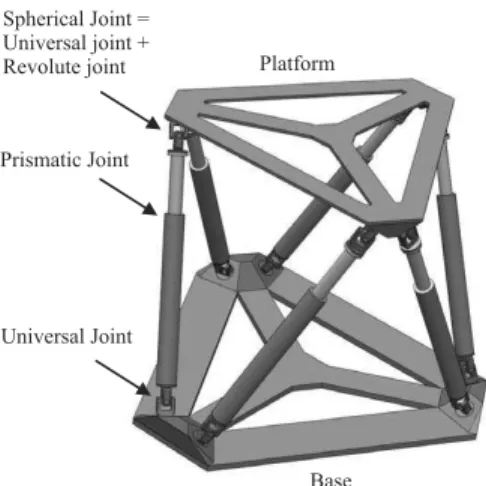
Most flight simulator adopt the Stewart platform as the motion base, which is composed of a moving platform linked to a fixed base through six extensible legs. Each leg is composed of a prismatic joint (i.e an electromechanical or electrohydraulic actuator), one passive universal joint and one passive spherical joint making connection with the base and the moving platform, respectively, as shown in Fig. 1.
Spherical Joint = Universal joint + Revolute joint
Universal Joint Prismatic Joint
Base Platform
Figure 1. The Stewart platform.
Most motion control schemes concerning flight simulator motion bases are focused on the washout-filter (Nahon and Reid, 1990), forward and inverse kinematics; and an independent joint linear controller is implemented for each actuator (Salcudean et al., 1994; Graf et al., 1998). On the other hand, the effects of the motion-base dynamics are ignored or a linearized model of motion-base dynamics is used (Idan and Sahar, 1996).
Inverse dynamics control (Sciavicco and Siciliano, 2005; Spong and Vidyasagar, 2006) is an approach to nonlinear control design whose central idea is to construct an inner loop control based on the motion base dynamic model which, in the ideal case, exactly linearizes the nonlinear system and an outer loop control to drive tracking errors
Paper received 3 December 2010. Paper accepted 9 November 2011. Technical Editor: Glauco Caurin
to zero. This technique is based on the assumption of exact cancellation of nonlinear terms. Therefore, parametric uncertainty, unmodeled dynamics and external disturbances may deteriorate the controller performance. In addition, a high computational burden is paid by computing on-line the complete dynamic model of the motion-base (Koekebakker, 2001). Robustness can be regained by applying robust control tecniques in the outer loop control structure as is shown in Becerra-Vargas et al. (2009).
In this context, this work presents the application of a control strategy applied in the outer loop of the feedback linearized system for robust acceleration tracking in the presence of parametric uncertainty and unmodeled dynamics, which is intentionally introduced in the process of approximating the dynamic model in order to simplify the implementation of this approach.
The forward and inverse kinematics and the dynamic model of six degrees of freedom motion base are briefly presented. Then, electromechanical actuator dynamics are included in order to obtain a full dynamic model.
The control strategy consists in introducing an additional term to the inverse dynamics controller which provides robustness to the control system. The robust control term is designed for a disturbance rejection problem via H∞ control, where the controller considers the uncertainties as disturbances affecting the linearized system.
Finally, standard methods to characterize the perfomance of a flight simulator motion base are presented and used to evaluate the performance of the controller.
Nomenclature
a = acceleration vector of the moving platform centre of gravity
bi = position vector of the i-th base point e = Cartesian coordinates tracking error vector
Fi = driving force generated by the i-th electromechanical actuator
g = acceleration vector due to gravity
Ip = moment of inertia matrix of the moving platform Jl,ω = Jacobian matrix relating toωandL˙i
Jl,q = Jacobian matrix relating toL˙i andq˙ Li = length of the i-th leg
M = mass of the moving platform (including payload)
c
M = simplified representation of the matrix M
b
N = simplified representation of the matrix N
pi = position vector of the i-th platform point (in moving platform frame)
q = Cartesian space coordinates vector qn = platform neutral position
(qp)i =ℜpi
(eqp)i = skew-symmetric matrix associated to(qp)i Qi = matrix depending on theith leg inertial properties R = position vector of the centre of gravity
e
R = skew-symmetric matrix associated withR
ℜ = rotation matrix of moving platform frame relative to base platform frame
si = unit vector along the direction of the i-th leg t = translation vector of the upper platform centroid,
(x, y, z)
u = robust control vector
Vi = vector depending on the i-th leg dynamic properties w = uncertainty vector
Greek Symbols
Θ = Euler angles vector,(φ, θ, ψ)
ω = angular velocity vector of the moving platform ωb = bandwidth of the flight simulator motion base α = angular acceleration vector of the moving platform τi = driving torque generated by theith electromechanical
actuator
Subscripts
i = Relative to actuatori
Superscripts
T = Represents transposition
Motion Base Kinematics and Dynamics
The Newton-Euler approach (Dasgupta and Mruthyunjaya, 1998) was adopted to calculate the Stewart platform nonlinear dynamic model in cartesian coordinates. The cartesian space coordinatesqare defined as
q=htT ΘTiT
, (1)
where t = [x y z]T is the translation vector of the moving platform centroid andΘ = [φ θ ψ]Tis the Euler angles vector defining its orientation.
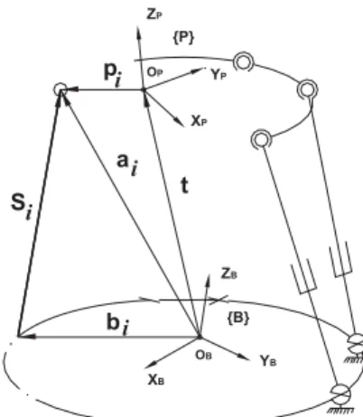
The leg vector with respect to the inertial base frame{B}, as shown in Fig. 2, can be denoted as
Si=ℜpi+t−bi (2)
Equation (2) represents the inverse kinematics problem in the sense one can compute the legs’ lengths, i.e., norms ofSi, from the given position (t) and orientation (ℜbeing function ofΘ) of the platform.
{P}
{B} ZB
OB
XB
YB
ZP OP
XP
YP
p
S
b a
t
i
i i
i
Figure 2. UPS Stewart platform.
The forward kinematics problem comprises the determination of the position and orientation of the platform from the given actuator lengths. It is observed from Eq. (2) that the forward kinematics problem involves solving six simultaneous nonlinear equations for the values of the six unknown variables representing the position and orientation of the platform. Consequently, iterative numerical methods are employed to solve the set of nonlinear equations (Nguyen et al., 1993).
Kinematic analysis of the legs can be derived from Eq. (2). Dynamic analysis of the legs can be derived taking force and moment balance of each leg (left side of Figure 3) and then combining both equations. Thus, one gets
(Fs)i=Qi¨t−Qi(˜qp)iα+V
i−Fisi (3)
where (Fs)i is the force applied to the leg i by the upper platform, Qi depends on the ith leg inertial properties and Videpends on theith leg dynamic properties.
Similarly, force and moment balance on the moving platform (right side of Figure 3) can be written as (with no external forces):
Ma=Mg− 6 X
i=1
(Fs)i (4)
and
MR×g− 6 X
i=1
[(qp)i×(Fs)i] +
6 X
i=1
fi=
Ipα+ω×Ipω+MR×a;
(5)
Figure 3. Vector analysis - Motion base.
Substituting the expression for (Fs)i from Eq. (3) into Eqs. (4) and (5) and then combining them, one gets
Mt(q)¨q+Ct(q,q˙) +Bt(q˙) +Gt(q) =Jl,ωF (6)
where:
Mt=Mp+Ma; Ct=Cp+Ca; Gt=Gp+Ga;
and
F= F1 F2 F3 F4 F5 F6 T.
The detailed elements of the above matrices are given in the Appendix. Information about derivation of the Stewart platform’s dynamic model is not detailed here since it is not the scope of this paper.
0.1 Inclusion of actuator dynamics
With the improvement in electrical servo actuation technology, there is a trend to use electrically driven motion systems instead of those hydraulically driven.
An electromechanical servo-actuator, shown in Figure 4, consists of a motor and an actuator driven by a servo-drive. As the closed loop bandwidth between the servo-drive and the servo-motor is much higher than that of the motion system, electrical dynamics can be ommitted and the mechanical dynamics is the only one considered. Thus, the motor torque can be considered proportional to the motor current.
Figure 4. Representation of the electromechanical servo-actuator.
The equation of motion of the electromechanical actuator (Figure 5) can be written in matrix form:
F=KaTm−DaL¨−BaL˙; (7)
where
Tm= τ1 τ2 τ3 τ4 τ5 τ6 T
.
L= L1 L2 L3 L4 L5 L6 T;
and where Da are the actuator inertia matrix, Ba is the actuator viscous damping coefficient matrix, and Ka is the actuator gain matrix, which are detailed in the Appendix.
Figure 5. Electromechanical actuator.
The relationship between the cartesian coordinates and joint coordinates can be written as
˙
L=Jl,qq˙
¨
L=Jl,qq¨+J˙l,qq˙ (8)
Substituting Eq. (8) into Eq. (7), one gets
F=KaTm−DaJl,q¨q−DaJ˙l,q−BaJl,qq˙ (9)
And substituting Eq. (9) into Eq. (6), the full dynamic model in cartesian coordinates results as
M(q)¨q+N(q,q˙) =uT (10)
where
N=C+E+G
M=K−a1hJl,ω−TMt+DaJl,qi
C=K−a1
h
Jl,ω−TCt+DaJ˙l,q+BaJl,qq˙
i
E=K−a1J−T
l,ωBt
G=K−a1J−l,ωTGt
Figure 6. Cartesian space control framework.
1. Motion Base Controller Design
A flight simulator control system stems from two frameworks. The first one is based on the legs lengths tracking control and is called joint space control (Salcudean et al., 1994; Graf et al., 1998). On the contrary, the second one is based on the position and orientation tracking control and is called cartesian space control (Becerra-Vargas et al., 2009; Koekebakker, 2001).
Joint space control does not seem suitable in inverse dynamic control due to the fact that joint space dynamic equations are more complicated compared with the cartesian ones in Eq. (10), moreover, the terms of the joint space dynamic matrices will still depend on the cartesian coordinates.
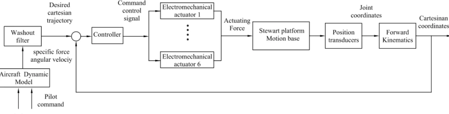
Cartesian space control was adopted in this study as shown in Fig. 6. The pilot responds to the simulator cues and tracking or disturbance tasks by driving the aircraft control surfaces, then aircraft’s response is calculated through an aircraft dynamic model.
Because of the limited motion envelope of the motion base, filtering (by washout filter (Nahon and Reid, 1990)) is required between the calculated aircraft trajectories and the commanded motion base trajectories. Then, the controller attempts to null the cartesian coordinate error by commanding a torque signal (voltage or current) to the servo-drive of the electromechanical actuator.
Thus, the force driving the motion base is governed by the equation of motion of the electromechanical actuator in Eq. (9).
Cartesian space control needs information of a 6 degrees of freedom sensor to measure the position and orientation of the platform. However, when only legs lenghts measurements are available, the forward kinematic problem must be resolved.
1.1 Imperfect compensation of the inverse dynamics control
As it is well known, inverse dynamics control (Sciavicco and Siciliano, 2005; Spong and Vidyasagar, 2006) is an approach to nonlinear control design whose central idea is to construct an inner loop control which, in the ideal case, exactly linearizes the nonlinear system and an outer loop control to drive tracking errors to zero. The global linearization of the motion base dynamics can be obtained by the inverse dynamics control
law:
uT =M(q)v+N(q,q˙) (11)
where M(q) and N(q,q˙) represent the matrices in Eq. (10) and:
v=¨qd+Kd˙e+Kpe, (12)
and where Kd and Kp represent the gain matrices and the tracking error is defined as
e=qd−q, (13)
where qd is the desired cartesian space coordinates. Now, substituting Eq. (11) into Eq. (10), and simplifying it, leads to the system of second-order equation:
¨
e+Kd˙e+Kpe= 0, (14)
where asymptotic stability is reached by choosing the matrices
Kd andKp as:
Kp= diagnωn21, ..., ω2n6o;
Kd= diag{2ς1ωn1, ...,2ς6ωn6} (15)
whereωniandςicharaterize the response of the tracking error in Eq. (14)
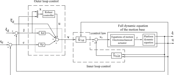
Practical implementation of the inverse dynamics control law in Eq. (11) requires the parameters of the matrices M(q) and N(q,q˙) to be accurately known, the matrices to be modeled accurately and to be computed in real-time. These requirements are difficult to satisfacy in practice. Model imprecision may come from parametric incertanties and purposeful choice of a simplified representation of the matrices M(q) and N(q,q˙) (unmodeled dynamics intentionally introduced). In other words, there will be always inexact cancellation (imperfect compensation) of the nonlinearities in the system due to these uncertainties also the burden of computing these matrices at each sample instant. Therefore, the control law in Eq. (11) can be rewritten as (Figure 7)
uT =Mc(q)v+Nb(q,q˙); (16)
where the termvis modified as:
Figure 7. Inverse dynamic control, imperfect compensantion.
and Mc, Nb represent simplified versions of M, N and are defined in Section III-C. The termu in Eq. (17) is included to overcome imperfect compensation effects, in this case, the simplification of the matrices M, N. The block that represents the full dynamic equation of the motion base in Fig. 7 corresponds to Eq. (10). Now, substituting Eq. (16) into Eq. (10) and simplifying it, one gets
¨e+Kd˙e+Kpe=w−u; (18)
where
w= (I−M−1Mc)v−M−1∆N
∆N=N−Nb (19)
The state space representation of the tracking error dynamics described by Eq. (18) is given as
˙
x=Ax+B(w−u), (20)
where the state vector x consisting of the error and its derivative is written as:
x= [ e ˙e ]T
, (21)
and where
A= (H−BK) , K= Kp Kd (22)
and
H=
0 I
0 0
B=
0 I
(23)
In this context, the termumust be designed to stabilize the tracking error dynamics defined by Eq. (20) in the presence of the incertaintyw, which represents the imperfect compensation effects. In the next section, the strategy will be designed in order to find this term.
1.2 Robust outer loop design byH∞ control
In order to useH∞control one needs to put the system in Eq. (20) into linear fractional transformation frame as shown in figure 8.
Figure 8. H∞control problem.
G(s) is the transfer function of the state space system defined by Eq. (20), andWe(s),Wd(s) andWu(s) represent the weighting functions diagonal matrices associated with the tracking error, disturbance and control signal, respectively (uncertaintywin Eq. (19) is considered as disturbance).
Then the H∞ suboptimal control problem is to find a stabilizing controllerK(s) which, based on the information in y, generates a control signaluthat counteracts the influence ofwe onez, thereby minimizing the closed-loop norm fromwe
toez to less than gamma via the selected weighting function matrices, that is
"
Wu(I+KG)−1KGWd
We(I+GK)−1GWd
#
∞ < γ (24)
1.2.1 Weights selection
problems in the algorithm used to synthetize the controller, it is necessary to place a pole very close to the origin in the left half plane, thusWe is given as
We(s) = s/Ms+ωb
s+ωbAs (25)
whereAs is chosen small to force tracking at low frequencies, Ms is the bound in high frequencies andωbis the bandwidth of the flight simulator motion base.
Wd is chosen to model the characteristic frequency of the disturbance and it is given as
Wd= Mds+ωb
s+ωb/Ad (26)
where Ad lower bounds the transfer functions in Eq. (24), penalizing the tracking error and the controller energy, respectively, whereasMd upper bounds the tranfer functions. As the disturbance (modeling error of inexact cancellation of the inverse dynamic control strategy, Eq. (19)) is generated through inverse dynamic computation, the bandwidth frequency is the same as the one of the motion system.
Wuhas to have the character of a high pass filter in order to reduce the effect of noise on plants outputs in high frequencies, thus
Wu(s) =s/Mu+ωb
s+ωbAu (27)
where Au normalizes the control signal (thus bounding the actuator signal) at low frequencies andMuupper bounds the control sensitivity function. Thus, the weighting functions matrices are given as:
We=
We(s)··· 0 ..
. . .. ...
0 ··· We(s)
;Wd=
Wd(s)··· 0 ..
. . .. ...
0 ··· Wd(s)
Wu=
Wu(s)··· 0 ..
. . .. ...
0 ··· Wu(s)
(28)
It is observed from Eq. (24) that the transfer functions, (I+GK)−1G and I+KG)−1KG are two-sided weighted functions, therefore the termsAs,Ad,Au andMs,Md,Mu
lower and upper bounds the spectrum of them.
1.3 Characteristics of the dynamic equations
Parallel manipulators motion bases have some drawback of relatively small workspace comparing to serial manipulators. In flight simulators motion bases, this is due mainly to the physical restriction in terms of position, velocity and acceleration of the actuators, e.g, for low frequencies motion, the velocity and position constraints limit the maximal attainable acceleration. Moreover, the high pass wash-out filter characteristics keep the motion system not very far away from the neutral position, to prevent the actuators from running out of stroke. Thus, the matrices Mc(q) and
b
N(q) of the control law in Eq. (16) can be approximated to constant ones without introducing large modelling errors.
Based on these constant matrices, calculation of the inverse dynamics becomes much simpler, reducing computation time significantly.
In this context, matrices Mc(q) and Nb(q), considered in the control law in Eq. (16), are defined at the neutral position as:
c
M(qn) =K−a1Jl,ω−T(qn)Mp(qn)
b
N(qn) =Gb(qn) =K−a1J−T
l,ω(qn)Gp(qn)
(29)
whereqnrepresents a neutral position and was chosen to be at half stroke of all the actuators,Mp(qn) is the inertia matrix (Eq. (31)) calculated at the neutral position, Gp(qn) is the gravity vector (Eq. (34)) calculated at the neutral positon and J−l,ωT(qn) is the jacobian (Eq. (38)) calculated at the neutral position. Coriolis and centrifugal forces, and leg effects, are not considered.
2. Controller’s Performance Evaluation
At present, only one standard method to characterize the performance of a motion system is known (Koekebakker, 2001). This is described in the AGARD advisory Report (Lean, 1979).
0 10 20 30 40 50 60
-8 -6 -4 -2 0 2 4
Time, s
Acceleration, m/s
2
x y z
(a) Acceleration Components
0 10 20 30 40 50 60
-0.5 0 0.5 1
Time, s
Angular Velocity, deg/s
x
y
z
(b) Angular Velocity Components Figure 9. Rejected take-off maneuver.
a frequency domain evaluation and the step acceleration response in time domain. For each degree of freedom, six describing functions can be calculated.
The primary describing function is the comparison of the response of the motion-base in the driven degree of freedom to the excitation signal (sine acceleration input) and the other five describing functions (crosstalk describing functions) the comparison of pure parasitic motion (motion in other than the degree of freedom excited) to the excitation signal (Grant, 1986). Furthermore, to evaluate the system in its normal operating mode, some standard maneuvers should be evaluated as well.
In order to evaluate the control strategy, the amplitude of the excitation signals (sine acceleration inputs, step acceleration inputs and the desired trajectories from the manouvers) was choosen to keep the motion base approximately 70% of the system limits in position, velocity and acceleration.
Desired aircraft trajectories were generated from a flight-simulation model of a Boeing 747-400 in the UTIAS (University of Toronto Institute for Aerospace Studies) research flight simulator, and then passed through the well-kwnon classical washout filter (Nahon and Reid, 1990) in order to obtain the desired motion base trajectories.
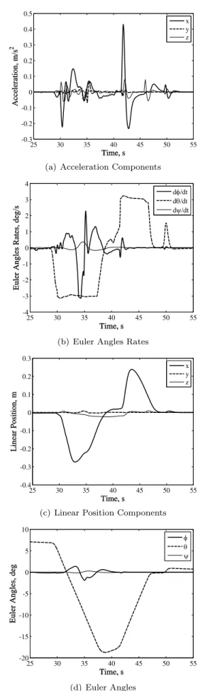
The aircraft rejected take-off maneuver acceleration and angular velocity as shown in Figure 9. From t = 10 seconds, the aircraft accelerates to takeoff (xforward direction ,ax= 4m/s2). After 20 seconds (t = 30 sec), the pilot decides to abort the take-off by applying brakes and retracting flaps as necessary (ax= -8m/s2). At t = 50 seconds the take-off has been aborted. The angular velocity of the aircraft is shown in Figure 9-b.
The filtered aircraft trajectory is shown in Figure 10 and represents the flight simulator motion base desired trajectory. It can be observed from Figure 10 that sustained forward acceleration (xacceleration component) is represented through a tilt coordination ( angleθ in Figure 10-d) and tilt angular velocity is limited to prevent the sensation of the angular rotation rate associated with the tilting (approx. 3 deg/s as shown in Figure 10-b).
3. Numerical Results and Discussions
The performance of the proposed controllers is verified by numerical simulations, and results are presented only for surge (x), heave (z) and pitch (θ) degrees of freedom. The Runge-Kutta fourth-order numerical integration method is used to solve the ordinary differential equation of the dynamic model. Computer codes are written in MATLAB. Geometric and inertial parameters of the motion base system are shown in Appendix B.
In order to yield a low-order controller it was considered that: the penalized output signals (y vector in Fig. 8) only correspond to the position error, and, the weighting functions are constants, i.e,y is a 6x1 vector andWe is a 6x6 matrix. Therefore, the weighting functions are given as:
25 30 35 40 45 50 55
-0.3 -0.2 -0.1 0 0.1 0.2 0.3 0.4 0.5
Time, s
Acceleration, m/s
2
x y z
(a) Acceleration Components
25 30 35 40 45 50 55
-4 -3 -2 -1 0 1 2 3 4
Time, s
Euler Angles Rates, deg/s
d/dt d/dt d/dt
(b) Euler Angles Rates
25 30 35 40 45 50 55
-0.4 -0.3 -0.2 -0.1 0 0.1 0.2 0.3
Time, s
Linear Position, m
x y z
(c) Linear Position Components
25 30 35 40 45 50 55
-20 -15 -10 -5 0 5 10
Time, s
Euler Angles, deg
(d) Euler Angles
We=
1/Ae ··· 0 ..
. . .. ...
0 ··· 1/Ae
;Wd=
Ad ··· 0
.. . . .. ...
0 ··· Ad
Wu=
1/Au ··· 0 ..
. . .. ...
0 ··· 1/Au
(30)
where Ae, Ad and Au were choosen as 0.008, 2 and 2.4, respectively.
With relation to the controller gains in Eq. (15), Koekebakker (2001) states the frequencyωishould not exceed human sensory thresholds and that it should ideally be sufficiently smooth and only require limited bandwidth (well below 1 Hz). In this paper, a bandwidth, ωi, of 2 Hz and a damping coefficient, ζi, of 1, were choosen necessarily to get the desired performance. Running through theγiteration technique (Skogestad and Postlethwaite, 2005) resulted in a suboptimal solution whenγ= 0.7415.
The ouput (So) and input (Si) sensitivity functions, and, the output (To) and input ( Ti) complementary sensitivity functions, defined from Figure 8, are shown in Figure 11.
10−2 10−1 100 101 102 −80
−70 −60 −50 −40 −30 −20 −10 0 10
Frequency (Hz)
Singular Values (dB)
Si Ti
(a) Input sensitivity functions
10−2 10−1 100 101 102
−80 −70 −60 −50 −40 −30 −20 −10 0 10
Frequency (Hz)
Singular Values (dB)
So To
(b) Output sensitivity functions Figure 11. Sensitivity functions.
Figure 11 proves the low-pass filter behaviour ofSi(input disturbance rejection) andSo(output disturbance rejection), and the high-pass filter behaviour of To (noise attenuation control in measuring output) andTi(noise attenuation control
in measuring input). So is less important in flight simulator motion bases considering no external forces acting on the motion base.
Acceleration step responses are shown in Figure 12. One can observe a damped response with a small time constant.
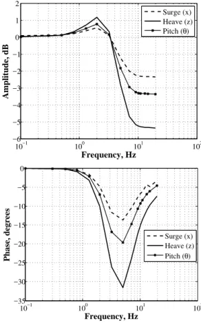
The heave, surge and pitch describing functions in Fig. 13 are very similar and present a flat response and bandwidth frequencies of approximately 20 Hz (tipically bandwidth frequency in high performance flight simulators).
0.2 0.3 0.4 0.5 0.6 0.7 0.8
0 0.2 0.4 0.6 0.8 1 1.2
Time, s
Normalized acceleration, m/s
2 x
z
θ
Figure 12. Acceleration step responses.
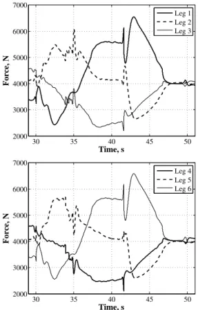
Crosstalks describing functions with the base driven in the surge direction (x) are shown in Figures 14. A rise occurs on parasitic pitch direction (θ) as the frequency increases, due possibly to the nonlinear coupling among the legs at high frequencies. Similar results were presented in the other directions, i.e, with the base driven in the pitch direction, a rise occurs on parasitic surge direction as the frequency increases. The acceleration response to the rejected take-off maneuver is shown in Figure 15. The driving torques supplied by the servo-motors of the servo-electromechanical actuators are presented in Figure 16. The motor angular velocities are shown in Figure 17. Similarly, the driving forces supplied by the actuators are shown in Figure 18.
One can observe from Figures 15, 16 and 18 short time peak accelerations, torques and forces (in 30 and 42 seconds approx), respectively. These peaks are produced due to the angular rate limiting that is applied in the washout filter (angular rate limiting can be observed in Figure 10-b). Angular rate limit leads to a very large angular jerk (derivate of acceleration), therefore large translation jerk is produced. This is important due to two reasons. One is a large jerk can lead to false cues, and the other is that if the magnitude of the jerk required is not considered, the motor may be undersized and the system won’t perform as required. A predictive motion cueing algorithm could avoid these false cues.
10−1 100 101 102 −6
−5 −4 −3 −2 −1 0 1 2
Frequency, Hz
Amplitude, dB
Surge (x) Heave (z) Pitch (θ)
10−1 100 101 102
−35 −30 −25 −20 −15 −10 −5 0
Frequency, Hz
Phase, degrees
Surge (x) Heave (z) Pitch (θ)
Figure 13. Describing function.
10−1 100 101 102
−120 −100 −80 −60 −40 −20
Frequency, Hz
Amplitude, dB
Pitch (θ) Heave (z)
10−1 100 101 102
−200 −150 −100 −50 0 50 100 150
Frequency, Hz
Phase, degrees
Pitch (θ) Heave (z)
Figure 14. Crosstalks describing function - Motion base driven in the surge direction (x).
30 35 40 45 50
−0.04 −0.03 −0.02 −0.01 0 0.01 0.02
Time, s
Acceleration errors, m/s
2
x z
(a) Surge (x) and heave (z) directions
30 35 40 45 50
−1.5 −1 −0.5 0 0.5 1
Time, s
Acceleration error, deg/s
2
θ
(b) Pitch direction (θ)
Figure 15. Rejected take-off maneuver - Acceleration errors.
30 35 40 45 50
5 10 15 20 25
Time, s
Motor Torque, N.m
Leg 1 Leg 2 Leg 3
30 35 40 45 50
5 10 15 20 25
Time, s
Motor Torque, N.m
Leg 4 Leg 5 Leg 6
30 35 40 45 50 −400
−300 −200 −100 0 100 200 300 400 500
Time, s
Angular Velocity, RPM
Leg 1 Leg 2 Leg 3
30 35 40 45 50
−400 −300 −200 −100 0 100 200 300 400
Time, s
Angular Velocity, RPM
Leg 4 Leg 5 Leg 6
Figure 17. Motor angular velocities.
30 35 40 45 50
2000 3000 4000 5000 6000 7000
Time, s
Force, N
Leg 1 Leg 2 Leg 3
30 35 40 45 50
2000 3000 4000 5000 6000 7000
Time, s
Force, N
Leg 4 Leg 5 Leg 6
Figure 18. Driving forces supplied by the actuators.
0.1 0.2 0.3 0.4 0.5 0.6
−0.5 0 0.5 1 1.5 2 2.5 3
Time, s
Acceleration, m/s
2
(a) Inverse dynamics control
0.1 0.2 0.3 0.4 0.5 0.6 0.7 0.8 −1
0 1 2 3
Time, s
Acceleration, m/s
2
(b) Robust inverse dynamics control
Figure 19. Step response in the surge (x) direction - Measured sensor noise.
4. Conclusions
In this paper, a control approach for the motion control of a flight simulator motion base was presented. The controller was implemented in the outerloop of the inverse dynamic control scheme in order to counteract imperfect compensation. Imperfect compensation was included intentionally by defining the motion base nominal dynamic matrices as constants. The approach was designed via H∞ theory. Controller performance evaluation was carried out through describing functions, step acceleration inputs and some standard manouvers. The controller presented robustness to bounded modelling error and measured sensor noise.
Acknowledgements
The author gratefully acknowledge the financial support provided by FAPESP (Sao Paulo State Foundation for Research Support - Brazil) through contract number 2005/25486-6.
References
Becerra-Vargas, M., E. Belo, and P. Grant (2009). Robust control of a flight simulator motion base. In AIAA Modeling and Simulation Technologies Conference, Chicago, IL, pp. 1–13. AIAA.
Theory 33(7), 993–1012.
Graf, R., R. Vierling, and R. Dillman (1998). A flexible controller for a Stewart platform. In Proceedings of the 1998 Second International Conference on Knowledge-Based Intelligent Electronic Systems, Adelaide-SA-Australia, pp. 52–59. IEEE.
Grant, P. (1986). Motion characteristics of the UTIAS flight research simulator motion-base. Technical report, University of Toronto - UTIAS, Toronto-Canada. Technical Note No. 261.
Idan, M. and D. Sahar (1996). Robust controller for a dynamic six degree of freedom flight simulator. In AIAA Flight Simulation Technologies Conference, San Diego, CA, pp. 53–64. AIAA.
Koekebakker, S. (2001). Model based control of a flight simulator motion system. Ph. D. thesis, Delft University of Technology, Netherlands.
Lean, D. (1979). Dynamic characteristics of flight simulation motion systems. Technical report, France. AGARD Advisory Report No. 144.
Nahon, M. and L. D. Reid (1990). Simulator motion drive algorithms - a designer’s perspective.Journal of Guidance, Control, and Dynamics 13(2), 702–709.
Nguyen, C., S. Antrazi, Z. Zhou, and C. Campbell (1993). Adaptive control of a Stewart platform-based manipulator. Journal of Robotic systems 10(5), 657–687.
Salcudean, S., P. Drexel, D. Ben-Dov, A. Taylor, and P. Lawrence (1994). A six degree-of-freedom, hydraulic, one person motion simulator. In Proceedings of the 1994 IEEE International Conference on Robotics and Automation, San Diego-CA, pp. 2437–2443. IEEE. Sciavicco, L. and B. Siciliano (2005).Modeling and Control of
Robot Manipulators (2 ed.). Londres: Springer-Verlag. Skogestad, S. and I. Postlethwaite (2005). Multivariable
Feedback Control (2 ed.). England: John Wiley & Sons Ltd.
Spong, M. and M. Vidyasagar (2006). Robot Modeling and Control (1 ed.). New York: John Wyley & Sons.
Appendix A
The matrices of the motion base dynamic model are given by:
Mp=
"
MI −MReℜω
MRe Ip−MReeR
ℜω
#
;
Ma=
6 X i=1
Qi −
6 X
i=1
Qi(qep)i
ℜω
6 X
i=1
(qep)iQi−
6 X
i=1
(qep)iQi(eqp)i
ℜω
(31)
Cp=
Mω×(ω×R) ω×Ipω+MR×(ω·R)ω
−
MRe MReRe−Ip
˙
ℜωΘ˙ (32)
Ca=
6 X i=1
(Vc)i
6 X
i=1
((qp)i×(Vc)i)
− 6 X i=1
Qi(eqp)i
6 X
i=1
(eqp)iQi(qep)i
˙
ℜωΘ˙
(33)
Gp=−hMMRg×gi; Ga=
6 X i=1
(Vg)i
6 X
i=1
((qp)i×(Vg)i)
(34)
Bt=
6 X i=1
(Vf)i
6 X
i=1
((qp)i×(Vg)i)−fi
. (35)
whereQidepends on theith leg inertial properties and
(V)i= (Vc)i+ (Vg)i+ (Vf)i, (36)
where (Vc)i and (Vg)i depend on the ith leg dynamic properties, and (Vf)i is the viscous friction force vector at theith leg joints, and where
ℜω=
CψCθ −Sψ 0
CθSψ Cψ 0
−Sψ 0 1
(37)
The motion base Jacobian is given as
Jl,ω=h s1 s2 s3 s4 s5 s6
q1×s1q2×s2q3×s3q4×s4q5×s5q6×s6
iT
, (38)
and the Jacobian that maps the cartesian coordinates into joint coordinates is given as
Jl,q=Jl,ωJω,q (39)
where
Jω,q=
I 0
0 ℜω
The matrices of the equation of motion of the electromechanical actuator are given as
Ka=
Ka ··· 0
.. . . .. ...
0 ··· Ka
;Da=
Da ··· 0
.. . . .. ...
0 ··· Da
;
Ba=
Ba ··· 0
.. . . .. ...
0 ··· Ba
(40)
where
Ka= 2πηp ; Ma= Jt4π2η
p2 ; Ba= B
t4π2η
p2
Appendix B
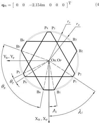
A symmetrical distribuition of joints on the payload are arranged as shown in Figure 20, where the anglesθB andθP and the upper and base platform radius values, rP and rB, respectively, are given in Table 1. The neutral position is choosen at half stroke of all the actuators, i.e.
qn= 0 0 −2.154m 0 0 0 T (41)
Figure 20. Platform and base leg points distribuition.
Table 1. Geometric and inertial parameters.
Parameter Value Parameter Value
θP 100◦ θB 20◦
rP 1.60 m rB 1.65 m