Francisco Paulo Lépore Neto
[email protected] Federal University of Uberlândia School of Mechanical Engineering 38408-902 Uberlândia, MG, BrazilMarcelo Braga dos Santos
[email protected] Federal University of Uberlândia School of Mechanical Engineering 38408-902 Uberlândia, MG, BrazilA Procedure for the Parametric
Identification of Viscoelastic Dampers
Accounting for Preload
Passive vibration isolators are usually made of viscoelastic materials. These materials have non-linear characteristics that change their dynamical properties with temperature, frequency and strain level. The vibration isolator’s mathematical modeling and optimal design require the prior knowledge of the stiffness and damping of the applied viscoelastic material. This work presents a dynamical characterization methodology to identify the stiffness and damping of three samples of viscoelastic rubber with hardness of 25, 33 and 48 SHORE A. The experimental apparatus is a one-degree of freedom vibratory mechanical system coupled to the viscoelastic damper. Sweep sine excitations are applied to the system and the resulting forces and vibration levels are measured. The amplitude of the excitation is controlled to achieve a constant RMS level of strain in the viscoelastic samples. The experimental results are obtained for conditions of no strain and with a 10% of pre-strain. The time domain data is post-processed to generate frequency response functions that are used to identify the damping and stiffness properties of the viscoelastic damper.
Keywords: viscoelastic, damping and complex stiffness
Introduction1
During the last five decades the usage of viscoelastic materials as passive vibration isolators and their characterization have been increasing. Jones (2001) states that the main contributions after 1960 have been the development of new applications and the development of methodologies for the characterization of viscoelastic material properties. Viscoelastic materials have been used in passive suspensions of heavy and light machines such as combustion engines, hard disks, bridges, large panels and other applications (Lakes, 1998).
As a consequence of the viscoelastic nature of rubbers, their dynamic behavior is significantly dependent on frequency, temperature and strain level. Moreover, due to the inclusion high content of additives within the compounds to optimize the mechanical performances of the rubber components, their dynamic behavior is markedly non-linear (Ramorino et al., 2003). Besides, the vibration isolators can present geometrical non-linearity. Therefore, mathematical modeling and optimal design require prior knowledge of the stiffness and damping coefficients of the applied viscoelastic material accounting for those complicating factors. However, in some cases, the properties can be estimated only in the actual damper, which imposes the development of a methodology to estimate the properties of the viscoelastic materials from tests with the entire damper device.
Tomlinson (1995) discussed the methodologies to evaluate the properties of viscoelastic materials. The main problems involved in these methodologies are the correct design of the test rig, the correct use of the instruments and the signal analysis. This author discusses how the flexibility of the test rig and its natural frequencies change the estimated values of the viscoelastic parameters.
This work presents a dynamical characterization methodology to identify the stiffness and damping of cylindrical viscoelastic specimens. The experimental apparatus is a one-degree of freedom vibratory mechanical system coupled to the viscoelastic damper. A harmonic excitation is applied to the system in order to measure the resulting forces and vibration levels. The experimental results are obtained at two static preload conditions for a frequency band between 0 Hz and 200 Hz. The time domain data is post-processed to generate the frequency response functions (FRF) which are used to identify the damping and stiffness properties of the viscoelastic
specimens. The methodology is applied to three samples of viscoelastic rubber with hardness of 25, 33 and 48 SHORE A.
Nomenclature
d = specimen diameter, mm F = force, N
h = specimen height, mm
= acceleration, m/s2
= velocity, m/s
= displacement, m
= elastic constant, N/m
∗ = complex stiffness, N/m
= damper damping coefficient, N/(m⁄s)
= mass, Kg
= storage modulus of viscoelastic material, N/m2 Greek Symbols
= cyclic frequency, ௗ ௦
= loss factor of the viscoelastic material
= geometric factor for the viscoelastic specimen Subscripts
e = relative to the excitation of vibratory system r = relative to the resonance peak
s = relative to the table suspension v = relative to the viscoelastic specimen c = relative to viscoelastic material
1 = relative to table the elastic coefficient of the suspension 2 = relative to the damping coefficient of the table suspension
Experimental Apparatus and Formulation
The moving disc (4) is used to apply dynamic loads to the specimens. It is connected to a single degree of freedom vibratory table driven by an electrodynamic shaker, as shown in Fig. 2. This configuration eliminates dry friction forces and prevents spurious motion, assuring that the vibratory motion takes place only in the horizontal direction.
Figure 1. Test rig diagram.
Figure 2 shows the complete experimental setup. The generalized coordinates xୱ and x୴ are used to represent the accelerations of the vibratory table and the moving ring (4) respectively. The acceleration of the latter can be assumed as being the same imposed to the viscoelastic specimens surfaces, as stated before, i.e. part (4) is assumed to be ideally rigid in the entire frequency band of the tests.
Figure 2. Experimental setup used in shear tests.
The vibratory table acceleration xୱ is measured by a piezoelectric accelerometer. The excitation force Fୣ and the force F୴ acting between the vibratory table and the specimen’s support (4) are measured by piezoelectric force transducers. A piezoelectric accelerometer, fixed to the support (4), measuresx୴. These signals are simultaneously acquired by an Agilent 35670A signal analyzer. Internally, the analyzer converts the voltage signals to engineering units. Thus the units of the signals from the load cells are converted to N and those from the accelerometers are converted to[m s⁄ ଶ]. The signal related to x୴ is used as reference to maintain constant the vibration amplitude over all excitation frequencies.
The physical model of the system presented in Fig. 2 was obtained using the free body diagram shown by Fig. 3, where Mୱ is the vibratory mass of the table and M୴ is the mass of the support (4) plus 1/3 of the specimens mass (Jones, 2001). F1 and F2 are the spring and damping forces generated by the vibratory table suspension, while K∗x
୴ is the force associated to the specimen complex stiffness.
By applying the second Newton’s law, one obtains the mathematical system model presented in Eq. (1), where Kୡ is the load cell stiffness.
Mxሷ= F− F− F− F= F− Kᇩᇭᇭᇪᇭᇭᇫሺx− xሻ
− Kx− Cxሶ
Mxሷ= F− K∗x= kሺx− xሻ− K∗x
(1)
Figure 3. Free body diagram of the vibratory system with the viscoelastic device.
Preliminary experimental tests indicated that the stiffness of the load cell is high enough to permit the hypothesis that xୱ≈ x୴ in the frequency band of the tests, and that Cୱ is small compared to the damping provided by the viscoelastic specimen. Under these assumptions the above equations can be reduced to Eqs. (2), which represent the motion of two single DOF systems:
Mୱ+ M୴xୱ+Kୱ+ K∗xୱ= Fୣ
M୴x୴ + K∗x୴= F୴
(2)
Assuming a steady-state harmonic excitation Fୣ= Fୣe୧ன୲ that will produce a response of the system as xୱ= Xୱe୧ன୲. From these the frequency response function (FRF) is obtained as follows:
ଡ଼౩
= ଵ
ିனమሺ
౩ା౬ሻାሺ౩ା∗ሻ (3)
Therefore, the complex stiffness K∗can be calculated using this FRF as follows:
K∗=
ଡ଼౩−Kୱ−Mୱ+ M୴ω
ଶ (4)
The same procedure can be used to analyze the motion of the mass M୴ resulting in an alternative expression for K∗, as follows:
K∗= ωଶM ୴+
౬
ଡ଼౬
(5)
It should be noted that, as the ratios Fୣ/Xୱ and F/X are complex owing to the phase lags between excitations and responses,
K∗ is a complex, frequency-dependent quantity. Since F
ୣ/Xୱ and
F୴/X୴ can be calculated from the measurements made with the sensors indicated in Fig. 2, the complex stiffness can be estimated from equations (4) or (5). Moreover, the complex stiffness is related to the complex elasticity modulus as indicated by Eq. (6) (Espíndola et al., 2005).
K∗= θE
ୡ1 + iηୡ (6)
In Eq. (6), θ is a constant dependent on the specimen geometry and on the test rig setup. Considering that cylindrical viscoelastic specimens are submitted to shear stress, Tomlinson (1995) suggests
E′ మRe
౩ K M Mω
η
మIm
౩
(7)
′
మ ೡ ೡ
మ ೡ
ೡ
(8)
It is observed in Eq. (7) and Eq. (8) the influence of the single DOF vibratory system in the estimative of the storage modulus and the loss factor, i.e. in Eq. (7) there are the influences of the stiffness and of the inertia M M, while in Eq. (8) only the inertia M
influences the storage modulus estimate. Moreover, it is important to notice that at higher frequencies the inertia influences will be higher and the estimate would be unsatisfactory.
Experimental Results
The experiments were conducted with two states of preload applied to the rubber specimens:
a) State 1: No preload was applied.
b) State 2: A prescribed displacement of 2.5 mm, equally distributed on the specimens due to the symmetry with respect to the moving ring, was applied as indicated in Fig. 4. This corresponds to a normal strain in each specimen ε . 0.104.
Figure 4. Schematic of preloaded specimens.
The excitation is controlled in order to sustain an acceleration of the specimen support (4) over all frequencies from 0 to 200 Hz, of the form x$ 15 sin2πft mm/s , since it had been verified that
at low frequencies the excitation force reaches values near 100 N, which is the upper limit of the shaker. The signal analyzer Agilent 35670A is used to control the acceleration x$producing a voltage
signal which is amplified to produce the excitation force through an electro-dynamical exciter. The signal analyzer is also used to estimate the transfer functions X/F and X/F. A group of settings
permits the adjustment of the waiting time, which is necessary for the PID control system to reach the steady state condition, and of the integration time, to reduce random errors in the transfer functions estimations. In this work the waiting time and the integration time were both adjusted to 100 periods of the excitation frequency. The frequency response functions were obtained with a resolution of 0.25 Hz, and are denoted as follows:
• X⁄F – is the receptance of the one degree of freedom
• X/F – is the receptance of the specimen support (4)
and the suspension formed by the viscoelastic specimens.
The experiments were conducted on three different viscoelastic rubber samples with different shore hardness. They are nominated as follows:
• Soft – Rubber with 25 shore A
• Medium – Rubber with 33 shore A
• Hard – Rubber with 48 shore A
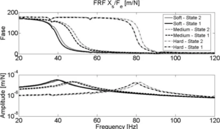
Error! Reference source not found. shows the transfer functions obtained with all specimens submitted to both states of preload, with 25oC room temperature, measured by a thermometer. The frequency band of interest has been defined as being 20 Hz to 120 Hz, in order to prevent noise originated from rigid body motions of the inertial table on which the test rig was mounted, and to magnify the differences between the rubber dynamical properties, for conditions without and with preload. It is important to point out that for hard rubber, the influence of the preload on the loss factor has been verified to be quite low for frequencies below 20 Hz.
It should be noted that the system natural frequency increases with the application of preload, as shown in Fig. 5. This is verified for all rubber hardness and it is more evident in the phase diagram. This means that the specimen stiffness increases with the preload compression level. Additionally, the resonance band widens for the soft rubber, indicating that the damping factor of the system also increases. It should be noted that this does not mean that the specimen viscous damping coefficient increases.
Figure 5. FRF’s from vibratory systems at all configurations.
Figure 6 shows the amplitudes of the transfer functions X/F
and X1/F, which are the receptance and the mobility curves,
respectively, for the system composed from the moving ring, part (4), and the viscoelastic suspension K∗. Assuming that the influence of the mass M can be neglected at low frequencies, these two
curves could be interpreted as indicators of the stiffness and damping coefficient of viscoelastic suspension. Thus, based on the results presented in Fig. 6, it is possible to conclude that the preload level increases the stiffness and the damper coefficient for all rubbers. This behavior is in agreement with that shown in Fig. 5, since the application of the specimen preload requires a higher force F to produce the same vibration level. Therefore, with a constant
mass, an increase of |F| should be related to higher values of the
Figure 6. FRF: Amplitude of the mobility ܄ ᇱ
܄
⁄ and receptance ܄/܄.
Parametric Identification of Complex Stiffness
The experimental FRFs are used to obtain the stiffness and damping properties of the specimens using a Voigt model, depicted in Fig. 7, associated to the viscoelastic behavior of the device. It should be noted that the parameters to be identified are not the material viscoelastic parameters; instead, the aim is to determine a set of parameters that represent an equivalent vibratory system with an additional suspension.
The identification procedure is done in two steps:
• Determine the stiffness K, damping coefficient C and
mass M of the table suspension without the viscoelastic
damper using a curve fitting method; all of them are constant parameters of a linear vibratory system. The curve fitting method minimizes the difference between the experimental and theoretical transfer functions using a direct search optimization algorithm.
• Adjust of the experimental receptance X/F with the
model of the vibratory system, now including viscoelastic damper, represented by the Voigt model parameters M, K and C.
The sum of the vibratory table suspension stiffness and the specimen stiffness can be used as a first guess, in the curve fitting algorithm, to estimate the stiffness values of the specimens. This hypothesis can be accepted because K and K are associated in
parallel and the load cell could be assumed as a perfectly rigid link between vibratory system and the viscoelastic device.
Lepore et al. (2008) have measured the vibratory table properties using a curve fitting methodology and obtained the following results:
• Mass: M 3.4 Kg
• Stiffness: K 50,194 N/m • Damping: C 5.05 Ns/m
Figure 7. Voigt model adopted to represent the viscoelastic damper.
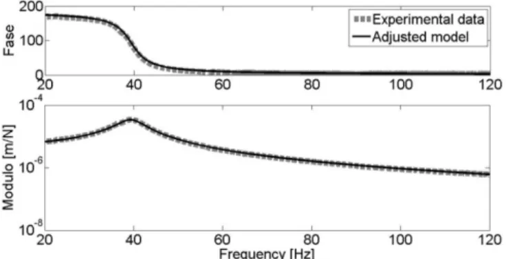
Figure 8 enables to evaluate the quality of the adjustment procedure by using the Voigt model for the soft rubber without preload. The total RMS error is 0.03% in the frequency band. It should be emphasized that the curve fitting process used is this paper is very dependent on the initial choice of state variables.
Figure 8. Adjusted Voigt model and the experimental data of the soft rubber without preload.
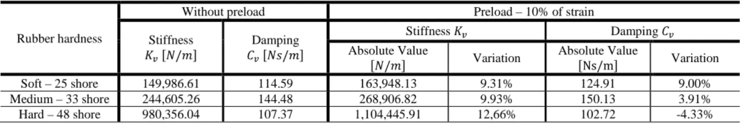
Table 1 shows the numerical results obtained for all the experiments. The stiffness of all rubbers shows a variation from 9.31% up to 12.66%, with respect to the damper without preload, which is an indication that the suspension becomes stiffer as the pre-strain increases. It is important to mention that Christensen (1982) states that creep is not perceptible in short time periods and that for steady harmonic conditions the dynamics effects are influenced by the initial strain, in which case it is possible to associate the preload with equivalent stiffness increment. Besides, the damping coefficient has a completely different behavior, i.e. the variation starts at 9% and decreases with the rubber hardness reaching a negative variation for the hardest one. The negative variation for the hardest rubber could be associated with the sharpness of the resonance peak that increases the error of the curve fitting method.
Table 2 shows the values of the natural frequency, damping factor and half bandwidth of the vibratory system with different rubber hardness and preload conditions. Bendat (1986) suggests that, for a light damped system, the half power bandwidth is expressed as B 2ξf. Therefore, small changes in the damping
coefficient using the preload produce a decrease in the sharpness of the resonance peaks, which means an increase of B. Analyzing the
half power bandwidth B and the damping factor ξ, for the soft
and medium rubbers, it is possible to affirm that the increment of the damper coefficient C is compensated by the increment of
the K, i.e. the benefits of the polymeric additives in increases the
damper coefficient, but is not sufficient to reduce the resonance peak sharpness.
Table 1. Materials properties estimated by curve fitting of the Voigt model.
Rubber hardness
Without preload Preload – 10% of strain
Stiffness
௩ /
Damping
௩ /
Stiffness ௩ Damping ௩
Absolute Value
/ Variation
Absolute Value
Ns/m Variation
Soft – 25 shore 149,986.61 114.59 163,948.13 9.31% 124.91 9.00%
Medium – 33 shore 244,605.26 144.48 268,906.82 9.93% 150.13 3.91%
Hard – 48 shore 980,356.04 107.37 1,104,445.91 12,66% 102.72 -4.33%
Table 2. Physical parameters of the tested vibratory systems.
Hardness of rubber
Without preload Preload – 10% of strain
Natural frequency [Hz]
Damping factor
Half power bandwidth [Hz]
Natural frequency [Hz]
Damping factor
bandwidth [Hz] Half power
Soft – 25 shore 39.50 0.074 5.846 40.75 0.077 6.276
Medium – 33 shore 47.39 0.075 7.109 49.21 0.075 7.382
Hard – 48 shore 79.47 0.027 4.291 81.99 0.027 4.427
Figure 9 shows the proposed one DOF Maxwell model to the vibratory system.
Figure 9. One DOF Maxwell model.
The values of K∗ have been calculated using Eq. (5) and the storage and the loss factor by means of Eq. (8). The number of elements, an association in series of a spring K and a damperC, necessary to represent the viscoelastic material as shown in the boxes of Fig. 9 are not fixed and vary with the material behavior. Jones (2001) suggests that it could be necessary more than 4 elements; however, the complexity of the fitting process increases also with the number of elements.
The model with one single element has complex modulus written as:
∗=1 + =+ ఠభభ
భାఠభ (9)
For the model with several elements the complex modulus is written as follow:
∗=
+
ఠమ
మ
మ
ାఠమ
మ
ୀଵ
+ ఠ
మ
మ
ାఠమ
మ
ୀଵ
(10)
Comparing the transfer function for Voigt, represented in Fig. 7, and Maxwell models, represented in Fig. 9 and modeled by Eqs. (9) and (10), it is possible to determine a correlation between the loss factor and the damper coefficient as follows:
=ೡఠ
ఏா (11)
௩= ఎఏா
ఠ (12)
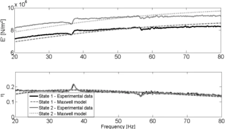
Figures 10 to 12 show the estimated values of E′ and η for each rubber obtained from experimental tests. These curves have been obtained using the parameters of the Maxwell models, as defined in Eq. (10). After that the storage modulus is obtained dividing K∗, by the geometric factor θ.
It is necessary to emphasize that differently from the resonant modes used to estimate the parameters the proposed methodology permits the estimation over a large frequency band in only one run. Christensen (1982) suggests that the resonant methods have as principal drawback the possibility to estimate the parameters only in vicinity of the natural frequencies of the test rigs. This disadvantage is overcome in the proposed methodology.
The mean values for the E′ obtained with Maxwell models are very close to the experimental data. The higher difference occurs with the elastic modulus of the hard rubber under 10% preload condition. The higher stiffness of the viscoelastic device in this condition can be the reason for this difference, at these values of viscoelastic devices stiffness the hypothesis that the supports are rigid cannot be verified at the full frequency band.
Figure 11. Estimated properties of the medium rubber.
Figure 12. Estimated properties of the hard rubber.
The elastic moduli, estimated or from experimental data, show that a preload makes the viscoelastic device stiffer. This behavior is verified in the whole frequency band and appears to be constant, i.e., the stiffness value of the preloaded specimens can be assumed as being a constant plus the stiffness of the specimens without initial strain. The peaks observed near 38 Hz, 58 Hz and 92 Hz in all experiments can be associated to local resonances of the linkage between the vibratory table and the viscoelastic device or to the viscoelastic device configuration. However, a more detailed study should be undertaken to explain this observation.
The loss factor η estimated for both states, with and without pre-load, is practically the same. Therefore, a carefull analysis of these curves should be done to evaluate the damper coefficientC୴, shown in Eq. (12). This is due to the dependence of the equivalent damper
C୴ to the elastic and dissipative moduli. So, any change in the values of equivalent damper can be due to a change in both moduli or in only one modulus, as can be seen in this paper. This behavior agrees with the analysis of half power bandwidth.
Conclusions
The methodologies to identify viscoelastic rubber’s physical properties by the Maxwell and Voigt models do not present significant differences in the signals treatment for the experimental conditions used in this work.
The equivalent damping identified by the Voigt model results the mean value of the viscoelastic damping coefficient that is valid at the resonance region of the vibratory system where the device is installed. Therefore, the Voigt model does not allow identifying the damping coefficient dependency on the excitation frequency.
The identification of the rubber physical properties using X୴/F୴ instead of Xୱ/Fୣ can be done without knowledge of the vibratory table properties used in the experimental tests. The proposed methodology when applied by using X୴/F୴ permits the identification of physical properties over a large frequency band in only one run. However, the same procedure when applied by using the Xୱ/Fୣ does not reach the same quality due to vibratory table dynamic behaviour. The proposed methodology estimates both storage and dissipative modulus of the viscoelastic material also with specimens under preload conditions.
Additionally, the Maxwell model allows identifying the loss factorηୡ, which is practically independent of the two preload levels used in the experiments. It is used to calculate the loss modulus of the viscoelastic material that is required for numerical analysis based on finite elements.
The preload value has important effect on the stiffness and damping properties of the device. This knowledge is important in the design of practical viscoelastic dampers used in machinery suspensions.
Additional works should be done to take into account nonlinear properties of the material and higher strain levels that appear in some devices. This would be done by reducing the size of specimens or by using another excitation device.
Acknowledgements
The authors acknowledge CNPq and FAPEMIG for their financial support.
References
Bendat, Julius S. and Pierson, Allan G., 2006, “Randon Data: Analysis and Measurement Properties”, 2nd Edition, John Wiley and Sons, New York.
Christensen, R.M., 1982, “Theory of viscoelasticity”, Academic Press, New York.
Espindola, J.J, Silva Neto J.M. and Lopes E.M.O., 2005, “A generalized fractional derivative approach to viscoelastic material properties measurements”, Applied Mathematics and Computation, 164, pp. 493-506.
Jones, David I.G., 2001, “Viscoelastic Vibration Damping”, First Edition, John Wiley & Sons Ltd, New York.
Lakes, Roderic S., 1998, “Viscoelastic Solids”, First Edition, CRC Press, New York.
Lepore, Francisco P. et al., 2008, “Identification of the Stiffness and Damping Dynamical Properties of a Vibration Isolator”, The 9th International Conference on Motion and Vibration Control, Munich, September.
Ramorino, G. et al., 2003, “Developments in dynamic testing of rubber compounds: assessment of non-linear effects”, Polymer Testing, Vol. 22, pp. 681-687.
Tomlinson, G.R. and Oyadiji, S.O., 1995, “Characterization of the dynamic properties of viscoelastic elements by the direct stiffness and master curve methodologies, part 1: design of load frame and fixtures”, Journal of Sound and Vibration, Vol. 186, pp. 623-647.
Responsibility Notice