Anderson Mossi
Federal University of Fronteira Sul 99700-000 Erechim, RS, BrazilMarcelo M. Galarça
[email protected] Federal Institute of Education Science and Technology of Rio Grande do Sul 96201-460 Rio Grande, RS, BrazilRogério Brittes
[email protected] Federal University of Rio Grande do Sul Department of Mechanical Engineering 90050-170 Porto Alegre, RS, BrazilHorácio A. Vielmo
[email protected] Federal University of Rio Grande do Sul Department of Mechanical Engineering 90050-170 Porto Alegre, RS, BrazilFrancis H. R. França
[email protected] Federal University of Rio Grande do Sul Department of Mechanical Engineering 90050-170 Porto Alegre, RS, BrazilComparison of Spectral Models in
the Computation of Radiative Heat
Transfer in Participating Media
Composed of Gases and Soot
Accurate combustion models are necessary to predict, among other effects, the production of pollutant gases and the heat transfer. As an important part of the combustion modeling, thermal radiation is often the dominant heat transfer mechanism, involving absorption and emission from soot and participating gases, such as water vapor and carbon dioxides. If the radiative heat transfer is not accurately predicted, the solution can lead to poor prediction of the temperature field and of the formation and distribution of the gases and soot. The modeling of the absorption coefficient of the gases is a very complex task due to its highly irregular dependence on the wavenumber. On the other hand, the absorption coefficient of the soot is known to behave linearly with the wavenumber, allowing for a simpler approach. Depending on the amount of soot, the more sophisticated and expensive gas models can be replaced by simpler ones, without considerable loss of accuracy. In this study, the radiative heat transfer for a medium composed of water vapor, carbon dioxide and soot is computed with the gray gas (GG), the weighted-sum-of-gray-gases model (WSGG), and the cumulative wavenumber (CW) models. The results are compared to benchmark line-by-line (LBL) calculations.
Keywords: radiative heat transfer, spectral gas models, soot radiation
Introduction1
The energy necessary to sustain the energy demand from industry and society is provided mostly by the combustion of hydrocarbons. However, environmental concerns with the pollution of gases emitted during the process require that new techniques are developed to control and reduce the levels of pollution. As such, accurate modeling of the soot formed in the process is important, because it strongly affects the temperature field and, in turn, the concentration of emitted gases, which is highly dependent on the temperature. In radiative heat transfer, emission from soot can be dominant, so the absorption and the emission from the participating gases, such as water vapor and carbon dioxide, may not play an important role when soot is present in a sufficient amount.
In the last few years, there has been a growing effort to predict the soot formation in combustion process. The main mechanisms of soot life are the nucleation, surface growth, agglomeration, and oxidation. Moss et al. (1988) proposed a model based on the premise that the soot reaction rates could be specified in terms of the mixture fraction. Experiments demonstrated that the acetylene is responsible for the surface growth and that the polycyclic aromatic hydrocarbons (PAH) initiate the soot nucleation. The oxidation is
performed mainly by the OH particles, but O2 molecules are
important in this process and have to be considered. Fairweather et al. (1992) subsequently proposed a simplified two-equation model for soot, where their model contains rate process for the nucleation, surface growth, agglomeration and oxidation. Experiments made by Sunderland et al. (1995) showed that the parameters used by Fairweather et al. (1992) are overestimated, which could result in a serious mistake in the amount of smoke produced by the flame. Wang et al. (2005) applied two radiation models to an
Paper received 31 October 2011. Paper accepted 10 January 2012 Technical Editor: Fernando Rochinha
enriched, propane-fueled, turbulent, non-premixed jet flame. The results showed that soot and spectrally radiating gas-phase species were distributed separately in the flame, and this segregation of radiating media strongly affected the radiative heat flux, flame structure and flame temperature. A numerical study of combustion in a liquid rocket engine was performed by Byun and Baek (2007). The simulation considered spray combustion at all speeds in the rocket engine with a non-gray finite-volume radiation model to investigate the radiation effect in turbulent combustion conditions, adding the soot formation and its effect on the radiation and flow field. Liu et al. (2004) studied the effects of radiation and the individual influence of gas and soot radiation on soot formation in counterflow C2H4SF diffusion flames by comparing the numerical results against available experimental data in the literature. On the other hand, gas models have been developed since the 1960’s, although the problem to compute radiation in gases can hardly be described as well as understood due to the highly complex dependence of the absorption coefficient of gases with the wavenumber spectrum. A discussion of the state of the art of gas modeling can be found in Galarça et al. (2011).
J. of the Braz. Soc. of Mech. Sci. & Eng. Copyright 2012 by ABCM April-June 2012, Vol. XXXIV, No. 2 / 113
coefficient, which can be considered the benchmark solution. The spectral data for water vapor, carbon dioxide and soot is obtained either from commonly employed engineering correlations or from detailed spectral database.
Nomenclature
aj = j-th gray gas corresponding blackbody weight, dimensionless
bj = polynomial coefficients of the WSGG model, units can vary C = absorption cross-section, m2/molecule
Dij = fractional gray gas, cm-1
Eb = blackbody total emissive power, W/m2
Ebη = blackbody spectral emissive power, W/(m
2 µm) fv = soot volumetric fraction, dimensionless H = Heaviside step-function, dimensionless Hj = wavenumber interval, cm-1
I = total radiative intensity, W/m2
Iη = spectral radiative intensity, W/(m2 cm-1) Jij = fractional gray gas intensity, W/m2
n = vector normal to the surface element, dimensionless N = molecular density, molecule/m3
P = pressure, N/m2
qR = radiative heat flux, W/m2
R
q& = radiative heat source, W/m3
( )
q&Rmax = maximum radiative heat source, W/m3 r = number of species, dimensionless
s = distance traveled by the radiation intensity, m
s = vector in the direction of the radiation intensity, dimensionless
Si = integrated intensity of line i, in (molecule cm-2)-1 T = temperature, K
uij = function of the cumulative wavenumber method, dimensionless
vij = function of the cumulative wavenumber method, dimensionless
w = cumulative wavenumber function, dimensionless x = position, m
Y = molar fraction, dimensionless
Greek Symbols
γ = half-width, cm-1/atm
δ = error, %
∆i = wavenumber interval, cm-1
ε = surface emissivity, dimensionless
η = wavenumber, cm-1
κ = absorption coefficient, m-1
κ′ = absorption coefficient per unit of partial pressure, m-1 atm-1
τ = optical thickness, dimensionless
Ω = solid angle, sr
Subscripts
air = relative to air
avg = relative to the average value
b = relative to blackbody g = relative to any gas i = relative to a spectral line i j = relative to j-th partial gray gas
max = relative to the maximum value ref = relative to the reference temperature s = relative to soot
self = relative to self-broadening
w = relative to wall surface
The Absorption Coefficient of Participating Gases and Soot
The absorption coefficient of participating gases is known by its strongly irregular variation with the wavenumber. According to Siegel and Howell (2002), for engineering applications, the absorption coefficient of the gases, κη, can be obtained with the Lorentz collision profile, given by:
(
)
∑
− += =
i i i
i i
S N
NC 2 2
γ η η
γ π
κη η (1)
where η is the wavenumber, N is the molar density of the absorbing
species, Cη is the absorption cross-section, Si is the integrated
intensity of line i, ηi is the line location, and γi is the half-width
given by:
(
)
ii n
i Y
T T Y
T T
, air 5
. 0 ref self, ref
1 γ
γ
γ −
+
= (2)
where Y is the molar fraction of the absorbing species, T is the temperature, γself is the self-broadening, γair is the air broadening half-width
.
The parameters required to obtain the spectral absorption cross-section can be obtained from databases such as HITRAN and HITEMP. For water vapor and carbon dioxide at high temperatures, the most appropriate database is the HITEMP, which is obtained for temperatures of 1000 and 1500 K. This means that extrapolation of the temperature for higher values will be more accurate when compared to extrapolation with data from HITRAN, which is obtained for a temperature of 296 K. Figure 1 shows the absorption coefficient for 10% H2O at 2000 K, depicting its characteristically complex dependence on the wavenumber. It should be observed that the figure presents only a narrow interval of wavenumber,
4000 cm-1 ≤ η≤ 4020 cm-1. The entire wavenumber spectrum is
formed by thousands of spectral lines, so that the spectral integration of the radiative transfer requires models to obtain solutions with a reasonable computational effort.
Figure 1. Absorption Coefficient of 10% H2O at 2000 K (From HITEMP
database 2008).
η
κη=7fν (3)
Equation (3) conveys that the dependence of the absorption coefficient with soot volumetric fraction, fν, is much less complex
than the behavior depicted in Fig. 1. Moreover, even in small quantities, soot radiation can be dominant over the radiation from gases, so one question that arises is: how accurate does the modeling of the participating gases need to be when the total radiation involves also the contribution of soot? Answering this question is the main goal of this paper.
Radiation Heat Transfer Modeling
The radiative transfer equation (RTE) for non-scattering media is given by:
η η η η
η κ κ
b
I I ds dI
+ −
= (4)
where Iη is the spectral radiation intensity, s is the distance
traveled by the radiation and Ibη is the spectral intensity of
radiation from a blackbody. In the right-hand side of the above equation, the first and second terms correspond, respectively, to
the increase and decrease of the spectral radiationintensity due to
absorption and emission in the medium. It should be noticed that the above equation neglects scattering of thermal radiation, since scattering from soot is negligible in comparison to its absorption and emission. Participating gases such as water vapor and carbon dioxide do not scatter. Equation (4) is subjected to the boundary conditions at the walls:
(
)
∫
< ⋅
Ω ⋅ −
+ =
0
1
s n
s
n d
I I
Iwη w bwη πw η
ε
ε (5)
where εw is the emissivity of a diffuse gray surface, Ω is the solid
angle, n is the vector normal to the surface (outward) and n⋅s is the cosine of the angle between any incoming direction s and the surface normal. In the right-hand side of Eq. (5), the first and second terms correspond, respectively, to emission and reflection of radiation from the surface element.
The solution of Eq. (4) to determine the radiation heat transfer requires integration in the space and the spectrum. In this study, the spatial integration will be carried out by the discrete ordinates method. The spectral integration will be performed with the gray gas (GG), the weighted-sum-of-gray-gases (WSGG), and the cumulative wavenumber (CW) models. These three models will be compared to the line-by-line (LBL) integration, in which Eq. (4) is integrated in every spectral line. Since the LBL integration involves no approximation in the spectral integration, it can be considered the benchmark for comparison.
Gray Gas Model
Several modern studies, especially in three-dimensional or combined mode problems, still consider the gas to be gray, for which the absorption coefficient is independent of the wavenumber. The integration of the RTE with the gray gas model yields:
b
I I ds
dI =−κ +κ
(6)
In solving the above equation, the absorption coefficient of the mixture is computed by the sum of the absorption coefficients of the gas and the soot phases:
s κ κ κ
κ= H2O+ CO2+ (7)
In this study, the gray gas absorption coefficients for H2O and
CO2 are correlated by Barlow et al. (2001), while the gray
absorption coefficient for the soot is calculated as suggested by Atreya and Agrawal (1998). The correlations are listed in Table 1. For H2O and CO2, the absorption coefficients are computed by
κg = κ′gPg, where κ′g is given in Table 1, Pg is the partial pressure of
the gas, and the index g represents either H2O or CO2.
Table 1. Curve fits for the absorption coefficient used in the gray gas model.
Species Absorption Coefficient
H2O and
CO2
(
)
∑
= = ′
5
0
/ 1000
i
i i
g c T
κ in m-1·atm-1
ci H2O CO2
c0 -0.23093 18.741
c1 1.1239 -121.31
c2 9.4153 273.5
c3 -2.9988 -194.05
c4 0.51382 56.31
c5 -1.8684×10⁻⁵ -5.8169
Soot κs = 1186fvT in m-1
The Weighted-Sum-of-Gray-Gases (WSGG) Model
The integration of the RTE, Eq. (4), with the WSGG model leads to:
b j j j j j
I a I ds dI
κ
κ +
−
= (8)
in which κj and aj corresponds, respectively, to the absorption
coefficient and the weighting factor for the j-th gray gas. Equation (8) is subjected to the following boundary condition:
( ) ( )
w b w jwj a T I T
I = (9)
where the weighting factor for the j-th gray gas is given by:
( )
( )
T Ed T E a
b b j
j
∫
∆= η
η ,η η
(10)
In the above equation, Ebη and Eb are, respectively, the spectral
and the total blackbody emissive power, computed at the medium temperature. Finally, the total intensity for N gray gases can be found by summing the intensities associated with each gray gas:
∑
=
=
N
j j
I I
1
J. of the Braz. Soc. of Mech. Sci. & Eng. Copyright 2012 by ABCM April-June 2012, Vol. XXXIV, No. 2 / 115
The WSGG model is frequently used with the correlations proposed by Smith et al. (1982, 1987) for the mixture of gases and soot. Although these correlations have been proved to be outdated, as discussed in Galarça et al. (2008), they continue to be extensively employed in engineering analysis, and were chosen to be used in this work to illustrate how they compare to solutions with modern gas data. The correlations are listed in Table 2 for a gas mixture with a molar ratio of 2:1 between water vapor and carbon dioxide. The local absorption coefficient of the j-th gray gas is obtained by
the product between the modeled coefficient κ′g and the total partial
pressure of water vapor and carbon dioxide, PCO2 + PH2O. The temperature dependent weights are approximated by a cubic polynomial function, given by:
∑
= − = 4 1 1 , , , i i i j g jg b T
a (12)
in which bg,ji is the polynomial coefficient obtained in Table 2,
where m and n are labels for gray gas and soot, respectively.
Coefficients of the WSGG model for gas mixtures, and for the soot. Source: Smith et al., 1982 and 1987.
Mixture, PH2O/PCO2 = 2
m κ′g,m
(m-1atm-1)
bg,j,1×101 bg,j,2×104
(K)
bg,j,3×107
(K2)
bg,j,4×1011
(K3)
1 0.4201 6.508 -5.551 3.029 -5.353
2 6.516 -0.2504 6.112 -3.882 6.528
3 131.9 2.718 -3.118 1.221 -1.612
Soot
n κs,n×10
-6 (m-1)
bs,1 bs,2×104
(K)
bs,3×107
(K2)
bs,4×1011
(K3)
1 1.00802 1.42 -7.7942 -0.38408 2.4166
2 3.2352 -0.42 7.7942 0.38408 -2.4166
For a mixture with soot, one more gray gas with null absorption coefficient is added (κg,0 = 0), corresponding to the transparent
windows of water vapor and carbon dioxide. Its correspondent temperature dependent weight is given by:
∑
= − = 3 1 , 0 , 1 i j g g a a (13)In the case of pure gas mixtures, the transparent windows do not contribute to the process, but in a mixture of gases with soot one should consider the emission and absorption of soot in the corresponding spectral regions.
For soot, the corresponding absorption coefficient is obtained by the product of the model coefficient and the soot volumetric fraction, and its weighting is given in an analogous way to Eq. (12). Thus, the absorption coefficient used in Eq. (7) for the mixture of the gases and soot is obtained by all possible combinations of the gas and soot absorption coefficients given in Table 2, defined as:
n s g,m
j κ κ ,
κ = + (14)
The temperature dependent weights for the mixture are defined as:
n s m g n m
j a a a
a = , = , , (15)
where the dimension of j is m×n.
The Cumulative Wavenumber Model
In this model, the entire spectral range of the absorption cross-section is divided into several gray gases and a non-decreasing function, called the cumulative wavenumber function, w, which is defined as:
( )
η =∫
η(
− η)
η0
, HC C d
C
w (16)
where H(C-Cη) is the Heaviside step-function, C is the absorption
cross-section of the gray gas, and Cη is the absorption cross-section.
Differentiation of Eq. (16) with respect to η yields:
( )
< > = ∂ ∂ η ηηη C C
C C C w for 0 for 1 , (17)
Thus, the integration of the wavenumber only in the regions where the gray gas coefficient C is larger than the true absorption cross-section is equivalent to integrating the derivative of the cumulative wavenumber function in the entire spectrum, according to:
( )
∫
( )
∫
∫
> ∞ = ∞∂ ∂ = 0 0 : ,
, η η
η η η
η
η d dwC
C w d C C (18)
The cumulative wavenumber method, proposed by Solovjov and Webb (2002), can be thought as a discretization in the fractional
gray gas wavenumbers (Dij) space. This interval Dij is defined as an
intersection of two wavenumber intervals, Hj and ∆i. The interval Hj
is the wavenumber region where the absorption cross-section is between two adjacent gray gases, that is:
{
C C C j n}
Hj= η: j−1≤ η≤ j, =1,L, (19)
And the interval ∆i is the wavenumber region divided in
subintervals:
[
i i]
i Ki= 1, , =1,L,
∆ η− η (20)
For a position s and all η ∈ ∆i, the difference between two adjacent gray gases can be viewed as a product of two functions:
(
Cj,s,η) (
wCj 1,s,η)
uij(s)νij(η)w − − = (21)
where the function vij(η) is the difference in the wavenumber
function evaluated at a reference thermodynamic state s*. Thus, function uij(s) can be defined as:
(
)
( )
(
(
η) (
) (
η)
)
η η η η , , , , , , , , , , ) ( * 1 * 1 s C w s C w s C w s C w v s C w s u j j j j ij j ij − − − − = ∆ = (22)
As shown in Solovjov and Webb (2002), the integration of the radiative spectral intensity Iη over the fractional gray gases Dij
intervals, using the cumulative wavenumber approach yields:
( )
[ ]
( )
( ) ( )
∫
=∫
∆ =ij i
D ij ij ij ij
s J s u v d I s u d
where Jij and uij are viewed as a fractional gray gas intensity and a
local correction to the fractional gray gas intensity, respectively. With this approach, Eq. (4) can be written as:
bij j ij j ij
J J s J
κ
κ +
− = ∂ ∂
(24)
where κj is the gray gas absorption coefficient, defined as:
1 −
= j j
j N C C
κ (25)
and Jbij is the fractional blackbody radiative energy source:
( )
∫
[
( )
]
[ ]
( )
∆
=
i
ij b
bij s I T s dv
J η ,η η (26)
The total intensity is obtained by the summation of the product between uij and Jij over all fractional gray gases, that is:
( )
=∑
( ) ( )
j i
ij ij sJ s
u s I
,
(27)
In the CW method, the spectrum is assumed to vary linearly with the concentration:
( )
η η(
η)
η C, w C/Y,
wYC = C (28)
It is also assumed that the intersections of the gray gases C with
the spectrum Cη+ C
* (the sum of the absorption cross-section with the absorption coefficient of gray particles) produce the same wavenumber intervals as the intersections of the gray gas C - C*
with the spectrum Cη, that is:
( )
η η(
η)
η , ,
∗
+ ∗ C =w C−C
wC C C (29)
For a mixture of gases and soot, Solovjov and Webb (2002) defined some approaches that can facilitate the use of this method: the superposition approach, the multiplication approach, and the hybrid approach. In this work, it is used the superposition approach, which assumes that the absorption cross-sections of the r species do not overlap and that the non-gray particles are piece-wise constant in the interval ∆i. Thus,
( ) ( )
∑
(
)
=
− +
− =
r
k
s i k
kC Y C
w r
C w
1
, / 1
,η η η (30)
where Cis = κη for η∈∆i, and κη is given by Eq. (3).
Results
In this section, it is analyzed the influence of soot in the radiative heat transfer as well as in the results of the different gas models. It is considered a one-dimensional geometry formed by parallel black walls placed at a distance of L = 1.0 m from each other. The position in the medium is defined by x, with the walls located at positions x = 0 and x = L. The space between the two walls is filled with a mixture of gases composed of 10% CO2 and
20% H2O. From the ideal gas mixture theory, the ratio between the
partial pressure of each species to the total pressure is equivalent to
its molar concentration, thus YCO2 = 0.1 and YH2O = 0.2. The medium
temperature varies according to the following equation:
( )
(
)
2max− 2 / −1
=T T x L
x
T s (31)
where 0 ≤ x ≤ L = 1.0 m, Ts = 500 K, and Tmax = 1000 K. With the
above relation, the temperature in the medium ranges from 500 K, in the vicinity of the surfaces, to 1000 K at the half distance
between the surfaces, which are assumed black (εw = 1). Four soot
volumetric fractions are considered: fv = 1×10⁻⁸, 1×10⁻⁷, 1×10⁻⁶
and 1×10⁻⁵. The last case, with fv = 1×10
-5
, is a higher than usual concentration in combustion of hydrocarbons, but it can represent situations where soot formation is intensified to supposedly increase the radiation effect.
Results are presented for the divergence of the radiative heat flux, in units of W/m3, which is one of the main parameters in the computation of radiation in participating media. It corresponds to the net rate of energy that leaves each element of volume in the medium per unit of volume, and is equivalent to the radiative heat source, but with opposite sign: dqR dx=−q&R.
When the divergence of the radiative heat flux is positive, it means that the element loses energy due to radiation. The divergence of the radiative heat flux is expected to be positive in the higher temperature regions of the medium and negative in the lower temperature regions of the medium.
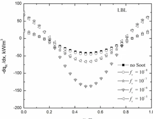
Figure 2. Benchmark results obtained with line-by-line calculations for the radiative heat source, q&R=−dqR dx.
Figure 2 shows the radiative heat source q&R=−dqR dx that
was obtained with line-by-line integration. In all cases, the radiative heat source was positive in the medium regions close to the surfaces, indicating that the gain of radiation from the hot regions of the medium exceeded the loss of radiation to the surfaces. Moving from the surfaces, x = 0 and x = L, towards the center, x = L/2, the radiative heat source decreased until it reached negative values, meaning that the loss exceeded the gain of radiation energy. Comparing the solutions for different soot volumetric fractions in Fig. 2, one can see that there is no significant difference between the case where there was no soot and the case with a very low
concentration (fv = 1×10⁻⁸). When the soot volumetric concentration
was increased to fv = 1×10⁻⁷, a considerable increase occurred in the
J. of the Braz. Soc. of Mech. Sci. & Eng. Copyright 2012 by ABCM April-June 2012, Vol. XXXIV, No. 2 / 117
gain of energy from the hot regions of the medium was compensated with an increased loss of energy to the surface. Figure 2 also shows that, when the soot concentration was incremented to fv = 1×10⁻⁶,
there was a strong increase in the radiation exchanged. In this case, the gas had only a minor contribution to the radiative heat transfer, which was soot dominated. Finally, for the situation where the soot concentration was as high as 1×10⁻⁵, the absolute value of the radiative heat source decreased in the center of the medium. In this situation, the medium became so optically thick that caused a decrease in the amount of radiation exchanged in the system. This behavior will be further explored later in this section.
Results for the radiative heat source obtained with the GG,
WSGG and CW models for the case with no soot, fv = 0, are
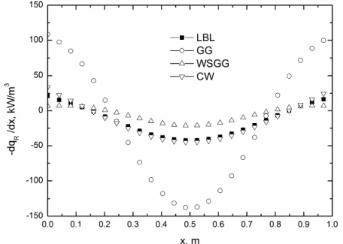
presented in Fig. 3. As can be observed, the GG model presents results with considerably large deviations from the LBL solution, leading to an overestimation of the radiation exchange in the system. The WSGG model presents results with a smaller but still noteworthy deviation from the LBL solution, which can be attributed to the fact that the correlations provided in Smith et al. (1982) were based on old gas data, which are known to be inaccurate. Finally, the CW model led to results that compared well with the LBL solution, with exception of the medium region close to the surfaces. It should be noted that the CW solution was built with the same spectral data of the LBL integration, and the model itself is based on a more sophisticated spectral analysis than the simpler approaches of the GG and the WSGG solutions. Additional comparison between the models can be made with the analysis of their relative errors, δ, which was computed in this work as:
(
)
100%max ,LBL
LBL , model ,
R R R
q q q
& & & −
=
δ (32)
where max
(
q&R,LBL)
is the maximum value for the radiative heat source for each volumetric fraction of soot.Figure 3. Comparison of the radiative heat sources (q&R=−dqR dx) obtained
with the LBL integration and the gas models with no soot (fv = 0).
Results for the maximum and average values of the relative error, δmax and δavg, are presented in Table 3 for all cases discussed in this study. The table indicates the high values of the relative errors for the GG and WSGG solutions, with maximum errors of 225.5% and 55.6%, respectively, for no soot. The CW model also led to a large maximum error, δmax = 29.5%, but the average error,
δavg = 7.6%, indicates that the model can be sufficiently accurate to
compute the radiation exchange for engineering computations when soot is not present.
Table 3. Maximum and average errors in each solution when compared with LBL model.
fν GG WSGG CW
δmax (%)
δavg (%)
δmax (%)
δavg (%)
δmax (%)
δavg (%)
0 225.5 137.5 55.6 23.1 29.5 7.6
1×10⁻⁸ 205.2 126.7 49.1 29.6 27.1 5.2
1×10⁻⁷ 123.5 74.2 44.7 26.9 17.5 7.2
1×10⁻⁶ 27.1 12.9 50.9 27.8 19.0 11.3
1×10⁻⁵ 14.4 7.9 87.6 39.2 297.7 151.7
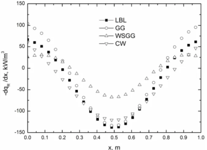
Figures 4 to 7 compares the solutions from the GG, WSGG and CW models with the LBL integration where the medium contains different amounts of soot. For small concentration of soot (fv = 10-8,
seen in Fig. 4), the general trends of the solution remained the same of the case without soot, but in general the deviation of the solutions to the LBL integration decreased, as can be observed in Table 3. By increasing the volumetric fraction of soot to fv = 10-7, as shown in
Fig. 5, the deviation of the GG and WSGG models to the LBL solution continued to decrease, especially for the GG model. As for the CW solution, although the maximum and average deviations did
not change considerably from the previous cases (fv = 0 and
fv = 10-8), the point of maximum deviation moved from the region
close to the surface to the center of the domain. Results for the highest amounts of soot, fv = 10-6 and fv = 10-5, are presented in Figs.
6 and 7, with major modifications in previous trends. First, results with the GG model became considerably more accurate in comparison to the LBL solution, in special for fv = 10-5, where the
maximum and average errors decreased to δmax = 14.4% and
δavg = 7.9%, respectively. On the other hand, the CW model led to considerably large deviations, δmax = 297.7% and δavg = 151.7%. This change in the trend can be attributed to soot radiation being
dominant for fv = 10-5. While the GG model allows a straightforward
approach to include soot in the integration of the radiative transfer equation, the CW model, proposed to deal with the highly complex dependence of the radiative properties of participating gases, requires a more elaborate approach that can fail when radiation is dominated by soot. Though not as critical as with the CW model, the WSGG model led to large errors when the amount of soot was increased.
Figure 4. Comparison of the radiative heat sources (q&R=−dqR dx)
obtained with the LBL integration and the gas models (fv = 10
-8
).
Figure 5. Comparison of the radiative heat sources (q&R=−dqR dx)
obtained with the LBL integration and the gas models (fv = 10-7).
Figure 6. Comparison of the radiative heat sources (q&R=−dqR dx)
obtained with the LBL integration and the gas models (fv = 10-6).
Figure 7. Comparison of the radiative heat sources (q&R=−dqR dx)
obtained with the LBL integration and the gas models (fv = 10
-5
).
One final discussion concerns the observation that the increase of soot from fv = 0 to fv = 10-6 led to an increase in the overall
radiation heat transfer, but for an even higher concentration of soot,
fv = 10-5, an opposite effect was observed, that is, the decrease in the
radiation transferred from the medium to the surfaces. For a more complete understanding of the phenomenon, Fig. 8 presents the radiative heat source in the mid-point between the two surfaces (x/L = 0.5) for different values of the optical thickness, τ = κL. As
seen, for τ→ 0, the radiative heat source tends to zero, as expected
for the limit of non-participating media. For τ→∞, in the limit of very thick media, the radiative heat source also tends to zero, since the media is so thick that radiation hardly escapes the point of emission. Figure 8 shows that the maximum absolute value of the radiative heat source occurs for τ≅ 3.0. Considering the radiation properties determined from the gray gas model, the optical
thicknesses based on the average absorption coefficient were τ≅ 5.5
and τ≅ 15.4 for the cases with fv = 0 and fv = 10-5, respectively,
explaining the decrease in the radiation exchange between the first and later cases. Thus, intensifying the formation of soot to increase radiation heat transfer can be beneficial only up to a certain point.
Figure 8. Radiative heat source (q&R=−dqR dx) at position x/L = 0.5 for
J. of the Braz. Soc. of Mech. Sci. & Eng. Copyright 2012 by ABCM April-June 2012, Vol. XXXIV, No. 2 / 119 Conclusions
This study considered the solution of the radiation heat transfer in a medium composed of soot and participating gases (water vapor and carbon dioxide). The radiative heat transfer equation was integrated with the use of three gas models, the gray gas (GG), the weighted-sum-of-gray-gas (WSGG) and the cumulative wavenumber (CW) models. The results of the three models were compared with the line-by-line (LBL) integration, which can be considered a benchmark solution. The GG and WSGG models were based on correlations that are widely employed in engineering analysis of radiation heat transfer, and led to results that shown considerable deviation from the LBL solution when the medium was composed solely of water vapor and soot. The inclusion of soot led to an improvement of the solutions provided by these two models, especially when radiation was dominated by soot. The CW model was built with the same spectral data of the LBL, leading to a satisfactory comparison for the medium composed solely of water vapor and soot, but led to large deviations when radiation was dominated by soot. The results presented show, therefore, that the choice of the gas model should take into account the amount of soot. More importantly, they reveal the need to develop new models or approaches to attempt a general treatment of the radiation heat transfer in media composed of constituents that present different spectral behavior, such as participating gases and soot.
Acknowledgements
The authors thank CAPES (Brazil) for the support under the Program CAPES/UT-AUSTIN, No. 28/2008. FHRF and HAV also thank CNPq for research grants 304535/2007-9 and 302503/2009-9, respectively, and for CNPq Universal Project 475237/2009-9.
The four last authors of this paper express their utmost gratitude for the opportunity to work with Anderson Mossi, who passed away a few weeks prior to his doctorate defense, in April of 2011. Anderson Mossi was a highly talented young researcher, who gained several friends in Brazil and USA with his great sense of humor and very positive attitude towards life. He is very much missed by all of us.
References
Atreya, A. and Agrawal, S., 1998, “Effect of Radiative Heat Loss on Diffusion Flames in Quiescent Microgravity Atmosphere”, Combustion and
Flame, Vol. 115, pp. 372-382.
Barlow, R.S., Karpetis, A.N. and Frank, J. H., 2001, “Scalar Profiles and NO Formation in Laminar Opposed-Flow Partially Premixed Methane/Air Flames”, Combustion and Flame, Vol. 127, pp. 2102-2118.
Byun, D. and Baek, S.W., 2007, “Numerical Investigation of Combustion with Non-Gray Thermal Radiation and Soot Formation Effect in
a Liquid Rocket Engine”, International Journal of Heat and Mass Transfer, Vol. 50, pp. 412-22.
Fairweather, M., Jones, W.P. and Lindstedt, R.P., 1992, “Predictions of Soot Formation in Turbulent, Non-Premixed Propane Flames”, Twenty-Fourth Symposium on Combustion, pp. 1067-1074.
Galarça, M.M., Maurente, A., Vielmo, H.A. and França, F.H.R., 2008, “Correlations for the Weighted-Sum-of-Gray-Gases Model Using Data Generated from the Absorption-Line Blackbody-Line Blackbody Distribution Function”, Proceedings of the 12th Brazilian Congress of Thermal Engineering and Sciences, Belo Horizonte, Brazil.
Galarça, M.M., Mossi A. and França, F.H.F., 2011, “A Modification of the Cumulative Wavenumber Method to Compute the Radiative Heat Flux in Non-Uniform Media”, Journal of Quantitative Spectroscopy & Radiative
Transfer, Vol. 112, pp. 384-393.
Hottel, H.C. and Sarofim, A.F., 1967, “Radiative Transfer”, Ed. McGraw-Hill Book Company, New York, United States of America, 520 p.
Jacquinet-Husson, N., 2008, “The GEISA Spectroscopic Database: Current and Future Archive for Earth and Planetary Atmosphere Studies”,
Journal of Quantitative Spectroscopy & Radiative Transfer, Vol. 109, pp.
1043-1059.
Liu, F., Guo, H., Smallwood, G.J. and Hafi, M.E., 2004, “Effects of Gas and Soot Radiation on Soot Formation in Counterflow Ethylene Diffusion Flames”, Journal of Quantitative Spectroscopy & Radiative Transfer, Vol. 84, pp. 501-11.
Moss, B.J., Stewart, C.D. and Syed, K.J., 1988, “Flowfield Modeling of Soot Formation at Elevated Pressure”, Twenty-Second Symposium on Combustion, pp. 413-423.
Rothman, L.S., Gordon, I.E., Barbe, A., Benner, D.C., Bernath, P.F. and Birk M., 2009, “The HITRAN 2008 Molecular Database”, Journal of
Quantitative Spectroscopy & Radiative Transfer, Vol. 110, pp. 533-572.
Siegel, R. and Howell, J., 2002, “Thermal Radiation Heat transfer”. Ed. Taylor and Francis, New York, United States of America, 868 p.
Smith, T.F., Shen, Z.F. and Friedman, J.N., 1982, “Evaluation of Coefficients for the Weighted Sum of Gray Gases Model”, ASME Journal of
Heat Transfer, Vol. 104, pp. 602-608.
Smith, T.F., Al-Turki, A.M., Byun, K.H. and Kim, T.K., 1987, “Radiative and Conductive Transfer for a Gas/Soot Mixture between Diffuse Parallel Plates”, Journal of Thermophysics Heat Transfer, Vol. 1, pp. 50-55.
Solovjov, V.P. and Webb, B.W., 2002, “A Local Spectrum Correlated Model for Radiative Transfer in Non-uniform Gas Media”, Journal of
Quantitative Spectroscopy & Radiative Transfer, Vol. 73, pp. 361-373.
Sunderland, P.B., Köylü, Ü.Ö. and Faeth, G.M., 1995, “Soot Formation in Weakly Buoyant Acetylene-Fueled Laminar Jet Diffusion Flames Burning in Air”, Combustion and Flame, Vol. 100, pp. 310-322.
Tashkun, S.A., Perevalov, V.I., Teffo, J.L., Bykov, A.D. and Lavrentieva, N.N., 2003, “CDSD-1000, the High-Temperature Carbon Dioxide Spectroscopic Databank”, Journal of Quantitative Spectroscopy &
Radiative Transfer, Vol. 82, pp. 165-196.