www.atmos-chem-phys.net/12/2037/2012/ doi:10.5194/acp-12-2037-2012
© Author(s) 2012. CC Attribution 3.0 License.
Chemistry
and Physics
Modelling future changes in surface ozone: a parameterized
approach
O. Wild1, A. M. Fiore2, D. T. Shindell3, R. M. Doherty4, W. J. Collins5, F. J. Dentener6, M. G. Schultz7, S. Gong8, I. A. MacKenzie4, G. Zeng9, P. Hess10, B. N. Duncan11, D. J. Bergmann12, S. Szopa13, J. E. Jonson14, T. J. Keating15, and A. Zuber16
1Lancaster Environment Centre, Lancaster University, Lancaster, UK 2NOAA Geophysical Fluid Dynamics Laboratory, Princeton, NJ, USA
3NASA Goddard Institute for Space Studies and Columbia University, New York, NY, USA 4School of GeoSciences, University of Edinburgh, UK
5Met Office Hadley Centre, Exeter, UK
6European Commission, Joint Research Centre, Institute for Environment and Sustainability, Ispra, Italy 7IEK-8, Forschungszentrum-J¨ulich, Germany
8Science and Technology Branch, Environment Canada, Toronto, ON, Canada 9National Institute of Water and Atmospheric Research, Lauder, New Zealand
10Department of Biological and Environmental Engineering, Cornell University, Ithaca, New York, USA 11NASA Goddard Space Flight Center, Greenbelt, MD, USA
12Atmospheric Earth and Energy Division, Lawrence Livermore National Laboratory, CA, USA 13Laboratoire des Sciences du Climat et de l’Environnement, Gif-sur-Yvette, France
14Norwegian Meteorological Institute, Oslo, Norway
15Office of Policy Analysis and Review, Environmental Protection Agency, Washington D.C., USA 16European Commission, Directorate General Environment, Brussels, Belgium
Correspondence to:O. Wild (o.wild@lancaster.ac.uk)
Received: 19 September 2011 – Published in Atmos. Chem. Phys. Discuss.: 11 October 2011 Revised: 28 January 2012 – Accepted: 6 February 2012 – Published: 21 February 2012
Abstract.This study describes a simple parameterization to estimate regionally averaged changes in surface ozone due to past or future changes in anthropogenic precursor emissions based on results from 14 global chemistry transport mod-els. The method successfully reproduces the results of full simulations with these models. For a given emission sce-nario it provides the ensemble mean surface ozone change, a regional source attribution for each change, and an esti-mate of the associated uncertainty as represented by the vari-ation between models. Using the Representative Concentra-tion Pathway (RCP) emission scenarios as an example, we show how regional surface ozone is likely to respond to sion changes by 2050 and how changes in precursor emis-sions and atmospheric methane contribute to this. Surface ozone changes are substantially smaller than expected with the SRES A1B, A2 and B2 scenarios, with annual global mean reductions of as much as 2 ppb by 2050 vs. increases of 4–6 ppb under SRES, and this reflects the assumptions of more stringent precursor emission controls under the RCP
scenarios. We find an average difference of around 5 ppb be-tween the outlying RCP 2.6 and RCP 8.5 scenarios, about 75 % of which can be attributed to differences in methane abundance. The study reveals the increasing importance of limiting atmospheric methane growth as emissions of other precursors are controlled, but highlights differences in mod-elled ozone responses to methane changes of as much as a factor of two, indicating that this remains a major uncertainty in current models.
1 Introduction
Increases in anthropogenic emissions of ozone precursors are believed to make a substantial contribution to the rising lev-els of surface ozone (O3) observed at many long-term
poor air quality and to economic and environmental damage. Understanding the reasons for its growth presents a consider-able challenge, as the balance of natural and anthropogenic, regional and global changes contributing to its growth varies greatly over the globe and remains poorly characterized (e.g. Lelieveld and Dentener, 2000; Sudo and Akimoto, 2007). While surface O3 is often considered a regional pollutant
that can be addressed with regional-scale precursor emission controls, it is also a global pollutant that can influence air quality over intercontinental scales (e.g. Akimoto, 2003; TF-HTAP, 2010). It remains unclear how regional emission con-trols aimed at reducing surface O3 may be offset by global
“background” O3 increases, by changes in the abundance
of longer-lived O3precursors such as methane (CH4) or by
changes in chemical processing or transport driven by future shifts in climate (Fiore et al., 2009; Jacob and Winner, 2009; TF-HTAP, 2010). Understanding the anthropogenic contri-bution to changes in surface O3requires a sufficiently good
understanding of the chemical and dynamical processes con-trolling O3and the sources and fates of its precursors to
ex-plain observed changes, and hence to reduce the current un-certainty in our estimates of future changes in O3affecting
air quality and climate.
This study explores the contribution of changes in anthro-pogenic O3 precursor emissions to changes in the regional
and global abundance of surface O3. It describes a simple
approach to quantify surface O3 changes based on regional
precursor emission changes derived from global chemical transport model simulations from a recent model intercom-parison. This is applied to past and future emission scenarios to explore the range of surface O3responses expected over
different parts of the world and to provide a source attribu-tion for these changes. The approach provides a measure of the uncertainty in the estimated responses as represented by the variation over the 14 independent models contributing to the study. We start by describing and evaluating the parame-terization used in Sects. 2–4, and test it with historical emis-sion changes in Sect. 5. We then explore a range of future emission scenarios in Sect. 6, quantifying the uncertainty in the expected O3changes and providing a regional source
at-tribution for these changes. We conclude by suggesting how the approach introduced here may be used to inform emission controls targeting air quality.
2 Model simulations and emission scenarios
Under the Convention on Long-range Transboundary Air Pollution (LRTAP), the task force on Hemispheric Trans-port of Air Pollution (HTAP) was established to develop a fuller understanding of the transport of a range of key air pollutants over intercontinental scales (TF-HTAP, 2007). A series of multi-model intercomparison experiments was co-ordinated by HTAP to provide a consistent quantification of intercontinental source-receptor relationships between major
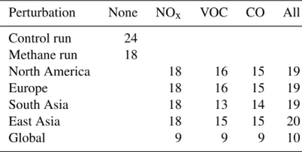
Table 1.Standard and additional simulations for the HTAP model intercomparison showing number of models contributing results for O3.
Perturbation None NOx VOC CO All
Control run 24 Methane run 18
North America 18 16 15 19
Europe 18 16 15 19
South Asia 18 13 14 19
East Asia 18 15 15 20
Global 9 9 9 10
industrialised regions. Global and regional models of atmo-spheric chemistry and transport were run with 2001 meteo-rological conditions and with best estimates of natural and anthropogenic emissions and a specified atmospheric abun-dance of CH4(1760 ppb), and these provided monthly mean
distributions of O3and aerosol and their precursors for the
year. A simulation with 20 % reduced atmospheric concen-trations of CH4was performed to determine the impacts of
CH4abundance on O3in each model, and this was followed
by a further series of runs with 20 % reductions in annual an-thropogenic emissions of the main O3 precursors, nitrogen
oxides (NOx), carbon monoxide (CO) and volatile organic
compounds (VOCs), individually and together, over each of the four main continental scale regions of interest in turn, see Fig. 1. Each model was run for one year, with additional time (typically six months) as spin-up. A response matrix was then generated to quantify the impact of each emission change over each source region on each receptor region in each model, and the resulting source-receptor relationships for O3 and its precursors are outlined in the HTAP
assess-ment reports (TF-HTAP, 2007, 2010) and are explored in fur-ther detail elsewhere (Sanderson et al., 2008; Shindell et al., 2008; Fiore et al., 2009).
For the present study, an additional set of four runs were defined with 20 % global emission reductions for each pre-cursor so that the effects of emission changes outside the four HTAP regions, the Rest-of-World response, can be con-sidered. The number of data sets from distinct models or model/meteorology combinations that were contributed for each simulation is summarised in Table 1. Each of these data sets provides the monthly mean spatial distribution of O3changes over the global domain for the specified emission
change, allowing continental-scale source-receptor relation-ships to be derived.
The models contributing to the HTAP intercomparison were run with their own best estimates of emissions for 2001 conditions. Recent studies of future surface O3 have
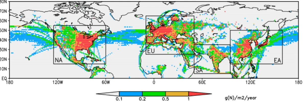
Fig. 1.Anthropogenic surface NOxemissions (g N m−2yr−1) for year 2000 from Lamarque et al. (2010) showing the HTAP source-receptor
regions considered here: N. America, Europe, S. Asia and E. Asia.
Three of the four scenario families introduced (A1, A2 and B2) show large increases in O3 precursor emissions that
reach or exceed a factor of two, and previous assessments of future air quality consequently show very large increases in future O3 that exceed 30 ppb in many regions by 2100
(e.g. Prather et al., 2003). In the present study we con-trast these with the new Representative Concentration Path-ways (RCP) generated for the Climate Model Intercompar-ison Project (CMIP5) simulations for the IPCC fifth assess-ment report along with harmonized historical emissions from 1850 to 2000 from Lamarque et al. (2010). Emissions of O3
precursors are available from 2000 to 2100 along each RCP pathway, and we use these along with the specified changes in atmospheric CH4abundance. The four RCP scenarios
rep-resent different assumptions about climate change mitigation measures, and are labelled by the levels of radiative forcing reached by 2100: RCP 2.6 (also referred to as RCP 3-PD), RCP 4.5, RCP 6.0 and RCP 8.5 (van Vuuren et al., 2011; Thomson et al., 2011; Masui et al., 2011; Riahi et al., 2011). Air pollution control policies are assumed to evolve under the different scenarios, and emissions of most O3
precur-sors decline by 2050, although more strongly in the cleaner RCP 2.6 scenario than in the high radiative forcing RCP 8.5 scenario, and with substantial differences in regional distri-bution. We note that the four RCP scenarios represent possi-ble future emission pathways, but have been developed inde-pendently and are governed by different assumptions about social, economic and political development. Differences in the treatment of CH4emissions, in particular, lead to large
differences in the atmospheric CH4concentrations used here,
and we show that this has important consequences for tropo-spheric O3.
3 Parameterizing ozone responses
In this study we use model results from the HTAP inter-comparison to quantify the impact of a realistic range of changes in anthropogenic precursor emissions on surface O3
on a global, regional and sub-regional basis. The approach involves scaling surface O3 responses derived from 20 %
emission reductions by the fractional emission change for a given emission scenario over each region for each precur-sor. For each model the HTAP results provide the monthly mean O3 change, 1O3(i,j,k), over each receptor region,k,
for a 20 % reduction in emissions, Eij, of each precursor, i, over each source region, j. The atmospheric CH4
abun-dance in these model runs was fixed at 1760 ppb, and so we are not able to explore the effect of CH4emission changes;
however, we use model runs with 20 % reduced CH4
abun-dance (1408 ppb) to determine the regional O3 response to
CH4 changes, 1O3m(k). The monthly mean O3 response
over each region,1O3(k), is then calculated by summing the
individual responses for each of the three precursors (NOx,
CO and VOC) over the five regions encompassing all global sources (N. America, Europe, S. Asia, E. Asia and Rest-of-World) and including the response from the change in global CH4abundance:
1O3(k)= 3
X
i=1
5
X
j=1
fij1O3(i,j,k)+fm1O3m(k) (1)
The scale factor for the O3 response to each regional
pre-cursor emission change, fij, is dependent on the emission scenario and is given by the ratio of the fractional emission change, 1Eij/Eij, to the 20 % emission change applied in the HTAP simulations:
fij=
1Eij
0.2×Eij (2)
Similarly, the scale factor for the CH4response,fm, is given
by the ratio of the global abundance change,1CH4, to the
20 % abundance change: fm=
1CH4
0.2× [CH4]
(3) These scale factors vary linearly with the size of the applied emission change or change in CH4 abundance. This
a) b)
1 2 3 4 5 6 7 8 9 10 11 12
Month of Year
0 0.2 0.4 0.6 0.8
Surface O
3
Reduction /ppb
All
0 0.5 1 1.5 2
Surface O
3
Reduction /ppb
NOx CO VOC Over N. America
Over Europe
1 2 3 4 5 6 7 8 9 10 11 12
Month of Year
0 0.5 1 1.5 2
Surface O
3
Reduction /ppb
Global
0 0.5 1 1.5 2 2.5 3
Surface O
3
Reduction /ppb
N. America Europe South Asia East Asia Rest of World Over N. America
Global Mean
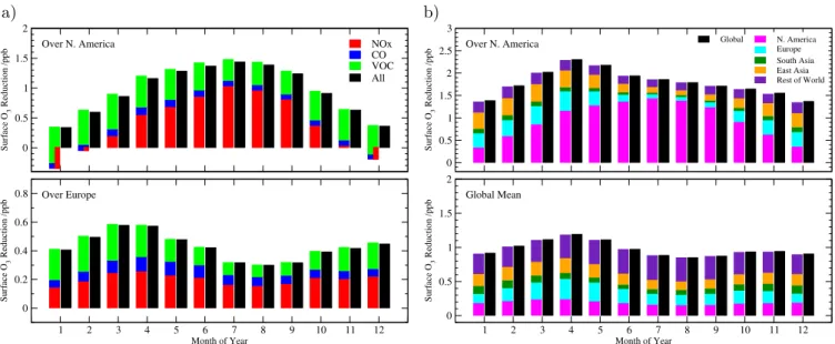
Fig. 2.Tests of linearity with the FRSGC/UCI CTM.(a)Sum of O3responses from 20 % reductions in anthropogenic NOx, CO and VOC
emissions from North American sources compared with responses from a combined 20 % emissions change, shown over the source region (upper panel) and a distant receptor region (Europe, lower panel). The contribution from NOxis negative over the source region in winter,
partly compensating for the effects of CO and VOC emissions.(b)Sum of O3responses from combined 20 % emission reductions over each
of the HTAP regions and over the rest of the world compared with the response from a global emission change, shown over a single region (N. America, upper panel) and over the globe (lower panel).
works well for small emission changes, and is applicable to larger changes with only minor modifications to account for the small degree of nonlinearity inherent in O3chemistry at
the continental scales considered here, described below. A major advantage of this combinatorial approach is its computational simplicity, allowing regional and global O3
changes to be explored for a wide range of different emission scenarios. Equation (1) can be applied to each atmospheric model in turn to generate a range of O3responses that reflect
the uncertainties in emissions, chemistry and transport over the contributing models. The approach can be used to deter-mine where the largest uncertainties arise, pinpointing model weaknesses, and to identify emission scenarios that would be of most interest to explore in further detail with full model simulations. In addition, the approach provides an immedi-ate regional source attribution for O3changes, something not
readily available from full model simulations without a tracer tagging scheme, such as that outlined in Grewe et al. (2010), or further sensitivity studies.
4 Testing the approach
To test the validity of the approach and quantify the errors involved, results from the HTAP intercomparison are supple-mented here by additional simulations using one of the con-tributing models, the Frontier Research System for Global Change version of the University of California, Irvine chem-ical transport model, FRSGC/UCI CTM (Wild et al., 2003).
Ozone responses due to individual precursor emission changes are used here in preference to those due to combined changes in NOx, CO and VOC emissions as many models
also included changes in aerosol in the combined runs. How-ever, changes in tropospheric photochemistry, particularly through the abundance of the hydroxyl radical, OH, couple the effects of these precursor changes such that the O3
re-sponses are not independent. Over the coarse temporal and spatial scales considered here the effects of the three individ-ual precursor emission changes are almost linearly additive, as noted in Fiore et al. (2009), with the fractional error,ǫc,
given by
ǫc= 3
P
i=1
1O3(i)−1O3c 1O3c
(4) where1O3cis the ozone response from the combined
emis-sion change. Figure 2 shows that the sum of the O3
re-sponses from each of the 20 % precursor emission changes in North American sources closely matches the response from the combined emissions change on a month by month ba-sis, both over the source region itself and over a downwind receptor region. The regional monthly responses from the sum of separate emission changes are marginally larger than those from the combined emission changes, by 2–7 % over the source region and by less than 2 % over receptor regions. Fractional errors are largest over the source region in winter where NOxemission reductions lead to enhancement in O3
is small in this season. NOx emission reductions provide
the largest O3response but lower the abundance of OH, and
hence the O3 response of CO and VOC reductions is less
when all three precursors are reduced together. Larger er-rors may be expected to occur on smaller spatial scales close to urban source regions which are more greatly influenced by rapid chemical processing and which may show strongly non-linear responses, but these effects are not seen at the con-tinental scales considered here, where behaviour is close to linear.
Rest-of-world O3 responses are required here to account
for changes in emissions outside the four HTAP regions. These are derived by subtracting the response due to emis-sions from each region from that of a global emisemis-sions change. To test the validity of this, additional simula-tions were performed with the FRSGC/UCI CTM apply-ing 20 % anthropogenic precursor emission reductions every-where outside the HTAP regions for each of the precursors in turn. The fractional error,ǫg, between the sum of the O3
re-sponse over the five individual regions and the O3response
to a global reduction,1O3g, is given by:
ǫg= 5
P
k=1
1O3(k)−1O3g 1O3g
(5) Figure 2 shows the difference between the sum of the re-gional and rest-of-world O3 responses and the response to
global emission changes. Over major source regions the re-sponse to local emissions dominates and shows a strong sea-sonality, while the global average response is more uniform. The differences are less than 2 % in all regions except for wintertime in Europe where they reach 4 % due to non-linear responses associated with the greater prevalence of O3
titra-tion in this region.
The 20 % emission perturbations applied in the HTAP studies were chosen to be small enough to give an approx-imately linear response while being sufficiently large to pro-vide robust signals in all models. However, the response of O3 to its precursor emissions is known to be non-linear
(e.g. Lin et al., 1988), and it is important to characterize where these non-linearities become significant. Scaling a 20 % emission reduction by a factor of five has been shown to underestimate the response to a 100 % reduction (Wu et al., 2009), and while this underestimation is relatively small for VOC emissions, generally less than 10 %, it can exceed a factor of two for NOxemissions (Wu et al., 2009; Grewe
et al., 2010), and shows a strong seasonal dependence (Wu et al., 2009). For this reason the sensitivity approach used in the HTAP studies is unsuitable for deriving a full source apportionment for O3. However, it does not preclude its use
in estimating the impact of less severe emission changes. To determine the limits of the linear scaling, additional simulations were performed with the FRSGC/UCI CTM for NOxemission changes ranging from complete removal to a
doubling of anthropogenic emissions. We focus on emissions from Europe, where deviation from linear behaviour is great-est due to higher latitudes and thus lower insolation which lead to substantial wintertime titration of surface O3.
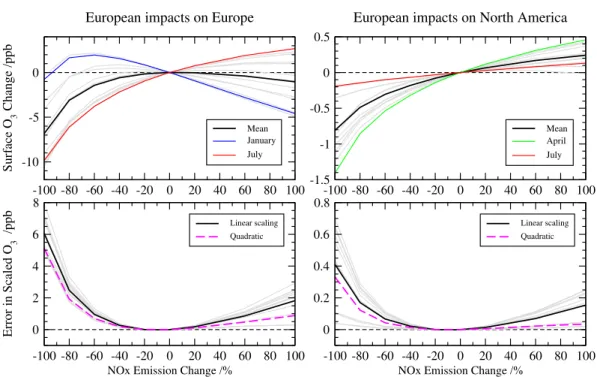
Fig-ure 3 shows the O3responses over the European source
re-gion and over a receptor rere-gion (N. America) along with the errors associated with linearly scaling a 20 % emission re-duction. Non-linear behaviour is clear, particularly over the source region where annual regional mean O3 is at a
max-imum in this model, and where additional wintertime titra-tion exceeds summertime productitra-tion for any further increase in NOx emissions. However, the nonlinearity is relatively
small for small emission changes, and the error in scaling 20 % changes remains below 1 ppb under emission changes of up to±60 %. In all cases a linear scaling leads to over-estimation of O3, reflecting the curvature of the O3response
shown in Fig. 3, and indicating that the magnitude of any O3 change will be underestimated for emission reductions
and overestimated for emission increases. Large departures from linearity are typically confined to emission reductions of more than 60 %, roughly equivalent to a return to NOx
emissions for 1950 over Europe and N. America and to 1970 emissions over South and East Asia. Over downwind recep-tor regions the nonlinear behaviour is weaker, and the frac-tional error is similar throughout the year so that the largest errors are present in April when the contributions from Eu-rope are greatest. Note that the errors identified here apply to the effects of NOxemission changes in isolation;
simulta-neous changes in CO and VOC emissions of a similar mag-nitude reduce the nonlinearity substantially. Complete re-moval of all anthropogenic emissions over Europe leads to an overestimate of 3 ppb over the source region using the lin-ear scaling compared with the 6 ppb overestimate seen here from removal of NOxemissions alone.
To account for the nonlinearity in O3 response to larger
NOxemission changes shown in Fig. 3, we replace the scale
factor, f, in Eq. (1) with a new factor, g, which has a quadratic dependence onf:
g=0.95f+0.05f2 (6)
This provides a small amount of curvature equivalent to an incremental reduction of 10 % in the O3 response for
each successive 20 % emission increase. The terms in this quadratic are chosen to provide a fit to the curves for the full CTM simulations shown in Fig. 3 (upper panels), and reduce the errors in the monthly O3 response by 20–60 %
for NOxemission changes of up to 60 %, as shown in Fig. 3
(lower panels). For emission reductions greater than 60 % this correction remains insufficient, and we do not expect the parameterization to work as well under these conditions. The approach is also insufficient to represent the response in source regions under titration regimes where an emission re-duction may lead to an increase in O3, as seen in January in
Fig. 3. Under these conditions we limit the O3response by
-100 -80 -60 -40 -20 0 20 40 60 80 100 -10
-5 0
Surface O
3
Change /ppb
Mean January
July
European impacts on Europe
-100 -80 -60 -40 -20 0 20 40 60 80 100 -1.5
-1 -0.5 0 0.5
Mean April
July
European impacts on North America
-100 -80 -60 -40 -20 0 20 40 60 80 100
NOx Emission Change /%
0 2 4 6 8
Error in Scaled O
3
/ppb
Linear scaling Quadratic
-100 -80 -60 -40 -20 0 20 40 60 80 100
NOx Emission Change /%
0 0.2 0.4 0.6 0.8
Linear scaling Quadratic
Fig. 3. Sensitivity of monthly O3 changes in the FRSGC/UCI CTM to the magnitude of European NOxemissions relative to current
conditions over the source region (left) and a downwind receptor region (N. America, right). Annual mean O3responses are shown in black and individual months in grey; months with the largest and smallest responses are highlighted. The lower panels show the error associated with linearly scaling a 20 % emission perturbation over the source and receptor regions (annual error in black, monthly errors in grey, scale factor “f”) and using a quadratic scaling (annual error in magenta, scale factor “g”).
and use the linear scalingf for emission increases, match-ing the responses seen in Fig. 3. Note that we only apply these changes for NOxemissions; non-linearity in the O3
re-sponse to CO and VOC emission changes has been shown to be much smaller (Wu et al., 2009), and we therefore retain the linear scale factor,f, for these precursors.
Previous studies have suggested that the O3 response to
CH4 emissions is approximately linear (Fiore et al., 2008).
However, we find that an additional CTM run applying a 20 % increase in CH4abundance gives an 11 % smaller O3
response over all regions than a run applying a 20 % CH4
decrease. Half of this 11 % reduction, about 5 %, reflects the feedback of CH4on its own lifetime (see, e.g. Prather,
1996), as a 20 % increase in CH4abundance requires a 5 %
smaller emission change than a 20 % decrease. Neverthe-less, it is clear that the response of surface O3to changes in
global CH4abundance is similar to changes in regional NOx
emissions, and we therefore choose to use the same scaling, given in Eq. (6), so that each successive 20 % increase in CH4
abundance gives a 10 % smaller O3increase.
In summary, the final expression used is given by Eq. (1) withfm=gmand with the scale factorfijfor precursori= NOxonly given by:
fij=
fij if1O3(i,j,k) >0 and1Eij>0
2fij−gij if1O3(i,j,k) >0 and1Eij<0 gij otherwise
(7)
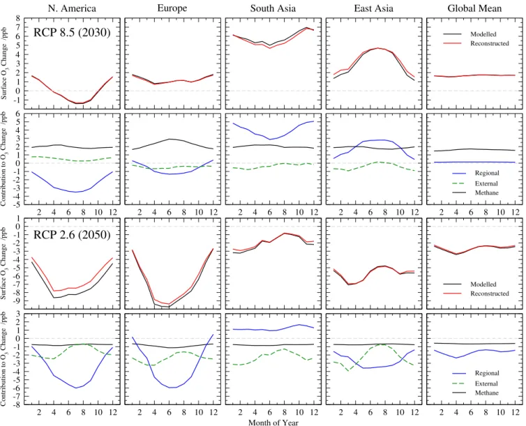
To provide a more critical test of the parameterization, we use it to reconstruct the results of new simulations with the FRSGC/UCI CTM using the RCP scenarios described in Sect. 2. Ozone precursor emission increases are largest in 2030 under the RCP 8.5 scenario, but the RCP 2.6 sce-nario shows large reductions by 2050, so we explore these two cases which encompass the extremes for the scenarios. A comparison between the monthly mean regional O3
re-sponses for a full simulation with the FRSGC/UCI CTM against that derived from the parameterization is shown in Fig. 4. In general the parameterization reproduces both the magnitude and the seasonality of the O3responses very well.
In the RCP 8.5 scenario there are small errors of up to 0.5 ppb in wintertime over East Asia, and this likely reflects in-creased titration of O3 associated with the relatively large
(65 %) increase in NOxemissions. Similarly, in the RCP 2.6
scenario the errors are largest in summertime over North America and Europe (reaching 0.8 ppb and 0.5 ppb, respec-tively), and this is associated with the relatively large NOx
emission reductions (70 % and 50 %, respectively) over these regions. Elsewhere, where emission changes are smaller, the magnitude and the seasonality of the O3responses in the full
simulations are matched very well, suggesting that the pa-rameterized approach used here is relatively robust.
-1 0 1 2 3 4 5 6 7 8
Surface O
3
Change /ppb
Modelled Reconstructed
2 4 6 8 10 12 -5
-4 -3 -2 -1 0 1 2 3 4 5 6
Contribution to O
3
Change /ppb
2 4 6 8 10 12 2 4 6 8 10 12 2 4 6 8 10 12
Regional External Methane
2 4 6 8 10 12
-9 -8 -7 -6 -5 -4 -3 -2 -1 0 1
Surface O
3
Change /ppb
Modelled Reconstructed
2 4 6 8 10 12 -8
-7 -6 -5 -4 -3 -2 -1 0 1 2 3
Contribution to O
3
Change /ppb
2 4 6 8 10 12 2 4 6 8 10 12 Month of Year
2 4 6 8 10 12
Regional
External Methane
2 4 6 8 10 12
N. America Europe South Asia East Asia Global Mean
RCP 8.5 (2030)
RCP 2.6 (2050)
Fig. 4. Monthly regional mean surface O3changes in the FRSGC/UCI CTM between 2000 and 2030 for the RCP 8.5 emissions (upper
panel) and between 2000 and 2050 for the RCP 2.6 emissions (lower panel). The upper row of each panel shows the estimated O3response compared with that from a full simulation, and the lower row shows the attribution of the O3response to global CH4changes (black) and to
emission changes inside (blue) and outside (green) the source region.
show the response to CH4abundance changes, regional
emis-sions changes, and emission changes outside the focus re-gion. This source attribution arises naturally from the simple combinatorial approach used here, and provides valuable ad-ditional insight without the need for tagged tracers in a full model simulation. The attribution reveals the extent to which the effects of regional emission reductions may be compen-sated by increases in emissions outside the region and in CH4, for example over North America in the RCP 8.5
sce-nario. While there is considerable redistribution of precursor emissions and surface O3under this scenario, the net change
in global surface O3 due to precursor emission changes is
close to zero throughout the year; in effect, the changes in global O3 are caused almost entirely by the elevated
abun-dance of atmospheric CH4 under this scenario. The
attri-bution also provides important insight into the role of inter-continental transport in contributing to regional surface O3
changes, which counteract the effect of regional emission reductions over North America under RCP 8.5, and the ef-fect of regional emission increases over South Asia under RCP 2.6.
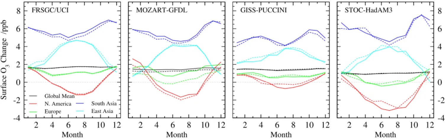
Finally, we demonstrate that the approach works well across a range of models. Modelled and estimated surface O3
responses from four different models simulating the RCP 8.5 2030 scenario are shown in Fig. 5. Each model is treated in-dependently, and the fractional emission changes along this RCP scenario are applied to the O3 responses from each
2 4 6 8 10 12 Month
-4 -2 0 2 4 6 8
Surface O
3
Change /ppb
Global Mean N. America Europe
2 4 6 8 10 12
Month
South Asia East Asia
2 4 6 8 10 12
Month
2 4 6 8 10 12
Month
-4 -2 0 2 4 6 8 FRSGC/UCI MOZART-GFDL GISS-PUCCINI STOC-HadAM3
Fig. 5. Monthly regional mean surface O3changes between 2000 and 2030 following the RCP 8.5 scenario with the FRSGC/UCI CTM, MOZART-GFDL CTM, GISS-PUCCINI GCM, and STOC-HadAM3 GCM (solid lines) and the parameterized estimate for each model (dashed lines).
Table 2.Chemistry transport models used to generate parameterization.
CAM-CHEM GEM-AQ INCA-LMDz MOZECH TM5-JRC
EMEP GISS-PUCCINI LLNL-IMPACT STOC-HadAM3 UM-CAM
FRSGC/UCI GMI MOZART-GFDL STOCHEM
in chemistry and transport and in assumptions about the dis-tribution and magnitude of emissions used in the present-day run. The estimates generally lie close to the true response for each model, with both the magnitude and seasonality of the responses reproduced well. The average root mean square (RMS) error in the estimates (0.26 ppb) is much less than the RMS variation between the models (1.2 ppb). We conclude that the approach used here is suitable for estimation of sur-face O3changes across the range of models contributing to
HTAP.
5 Anthropogenic contribution to historical trends
To explore the regional anthropogenic contributions to past O3 trends, monthly mean surface O3 responses were
ex-tracted from each of the 14 models which contributed a suf-ficiently complete set of results for the standard HTAP simu-lations to allow use with the parameterization (see Table 2). Where results for global emissions perturbations were un-available, the responses to rest-of-world perturbations were assumed to equal the ensemble mean responses for the mod-els that did contribute results. The response to changes in tropospheric CH4 abundance was also included. We use
the historical emissions of Lamarque et al. (2010) and de-rive regional and global surface O3responses for each model
by combining the responses for each precursor over each re-gion based on the fractional emission change from year 2000 emissions. While emission data are available from 1850, we focus on the period from 1960 to present to minimize the
er-rors introduced by applying very large emission reductions. Regional NOxemissions in 1960 were 40–45 % lower over
Europe and North America than in 2000, but were 75–80 % lower over South and East Asia, and the global CH4
abun-dance was 30 % lower.
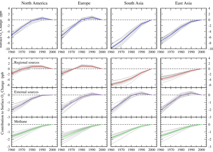
The changes in regional annual mean surface O3relative
to 2000 conditions are shown in Fig. 6. Regional increases since 1960 vary between 5 and 10 ppb, but the pathways differ substantially, with Europe and North America experi-encing increases of about 0.25 ppb yr−1until 1980, but then smaller increases that turn to a decline in the 1990s, while South and East Asia see steady increases of as much as 0.40 ppb yr−1. The uncertainty in these estimates as repre-sented by the variation between models is relatively small, with a 1σvariation of about±0.8 ppb since 1960. To test the robustness of these estimates, the FRSGC/UCI CTM was run with emissions representative of 1960 conditions. The error in estimates for the global and regional annual mean surface O3response is typically less than 0.1 ppb, and reaches a
max-imum of 0.25 ppb for East Asia, where NOxemissions were
75 % smaller in 1960 than 2000, and thus where we expect to underestimate the O3change. Nevertheless, this represents
an underestimate of less than 3 % of the calculated change of 8.4 ppb, and we conclude that the parameterization is ca-pable of representing the full model simulations under these conditions.
1960 1970 1980 1990 2000 -10
-8 -6 -4 -2 0 2 4
Surface O
3
Change /ppb
North America
1960 1970 1980 1990 2000 Europe
1960 1970 1980 1990 2000 South Asia
1960 1970 1980 1990 2000 -10 -8 -6 -4 -2 0 2 4 East Asia
-6 -4 -2 0 2 4
-6 -4 -2 0 2 4
-3 -2 -1 0
Contribution to Surface O
3
Change /ppb
-3 -2 -1 0
1960 1970 1980 1990 2000 -3
-2 -1 0
1960 1970 1980 1990 2000 1960 1970 1980 1990 2000 1960 1970 1980 1990 2000 -3 -2 -1 0 Regional sources
External sources
Methane
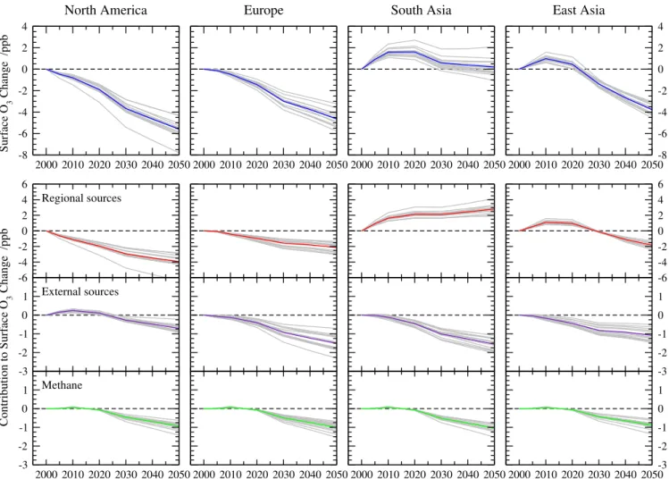
Fig. 6.Annual regional mean surface O3changes relative to 2000 over each HTAP region following historical precursor emission changes
between 1960 and 2000 (top row), and the contribution of regional anthropogenic sources, anthropogenic sources outside the region, and global methane changes (bottom row). Individual model responses are shown in grey and the mean of all 14 models is coloured.
changes on an annual mean basis. For Europe and North America the changes in regional and external precursor emis-sions have made a similar contribution since 1960, about 2 ppb, although this masks the faster rise and subsequent drop of O3from regional sources. Over South and East Asia,
re-gional emission changes contribute 4–6 ppb, more than 50 % of the increase. Increases in atmospheric CH4contribute to
all regions relatively uniformly, averaging 1.5–1.9 ppb since 1960, and this contributes about one third of the O3increase
seen over Europe and North America. Note the substantial uncertainty in the response to CH4reflected in a factor of two
difference between the most and least sensitive models, about
±0.75 ppb since 1960. This reflects differences in chemical environment, particularly in the abundance of OH, as noted elsewhere (e.g. Fiore et al., 2009). Nevertheless, the contri-bution to the uncertainty in the total O3changes since 1960
remains small, only about 0.1 ppb of the 1σ variation, sug-gesting that models with stronger O3responses to CH4have
weaker responses to other precursors.
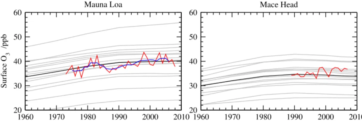
These surface O3changes due to growth in anthropogenic
precursor emissions are compared with observed surface O3
trends by extracting O3 responses at sites with long-term
measurements, see Fig. 7. The ensemble annual mean sur-face O3 matches the observations reasonably well at each
location, but the large spread over the different models (as much as±16 ppb at Mauna Loa) indicates that this apparent skill is somewhat illusory, hiding differences in annual and diurnal cycles as well as systematic biases due to process representation in the models and to sampling location on the different model grids. The general growth in O3is matched
well at Mauna Loa, remote from the main source regions considered here, with an average increase in O3 of about
1960 1970 1980 1990 2000 2010 20
30 40 50 60
Surface O
3
/ppb
1960 1970 1980 1990 2000 2010 20
30 40 50 60
Mauna Loa Mace Head
Fig. 7. Annual mean surface O3trends at Mauna Loa and Mace Head between 1960 and 2010 for individual models (grey) and ensemble
mean (black) against annual mean observed surface O3(red). The 5-year running mean of the observations at Mauna Loa is shown in blue.
in the models. The contribution of CH4increases in the
mod-els averages 0.05 ppb yr−1over this period, about 40 % of the trend at this site.
Closer to major continental regions the modelled trends are less well supported by observations. Unfiltered mea-surements at a coastal site, Mace Head, show an increase of about 0.17 ppb yr−1between 1989 and 2007, and trends in clean baseline air at this site are thought to be as high as 0.31 ppb yr−1 (Derwent et al., 2007). Modelled O3 shows
a positive trend of 0.08 ppb yr−1in the 1980s, but the trend turns negative after the 1990s, reflecting reductions in Eu-ropean emissions, and averages −0.03 ppb yr−1 over the measurement period. In the 1990s, this trend is driven by the dominance of European and North American contribu-tions (−0.03 and−0.04 ppb yr−1, respectively) over the
con-tributions from Asia and from global CH4 changes (each
0.02 ppb yr−1). The difference from the observed trend may
reflect weaknesses in emission assessments, but it may also reflect the spatial redistribution of emissions within regions which is not represented here (Vautard et al., 2006), or changes in shipping emissions which may have a substantial impact on coastal regions (e.g. Collins et al., 2008). Changes in natural sources, compounded by significant interannual meteorological variations, may also contribute to this dis-crepancy, and the influence of stratospheric O3is thought to
be significant (Hess and Zbinden, 2011). Further studies at regional scales accounting for spatial emission changes and meteorological variability are required to explain O3changes
at these continental locations, as previous studies have noted (e.g. Jonson et al., 2006).
6 Application to future trends
We now apply the parametric approach to explore changes in regional surface O3along the four RCP emission
scenar-ios. We do not account for any changes in climate, which would differ along the scenarios, but focus on the effects of anthropogenic precursor emission changes alone.
Emis-sion changes by 2100 are large along several of the scenar-ios, so we focus on the period between 2000 and 2050, when changes are smaller and the resulting error in our estimates is less. The ensemble regional mean changes are presented in Fig. 8, and changes by 2050 are summarized in Table 3 along with an estimate of the uncertainty as represented by the 1σ variation over the models. Under all four scenarios surface O3 falls over Europe and North America, although
this fall is reversed over Europe after 2020 along RCP 8.5, driven not by increasing regional emissions but by increas-ing atmospheric CH4. Surface O3increases over South Asia
in all scenarios, although there is a large difference between RCP 8.5, where increases of more than 5 ppb are seen by 2050, and RCP 6.0, where changes are close to zero. Over East Asia there is also a large variation, with increases in O3until 2020 but subsequently decreases under the RCP 2.6
and 4.5 scenarios. It is clear that under all RCP scenarios except RCP 6.0 the greatest increases in surface O3are over
South Asia, and the large increases here are a major concern given the high population of the region and the influence of the region on wider tropospheric composition through strong convective lifting associated with the South Asian monsoon. For comparison, the O3 responses along the SRES
sce-narios used in previous studies are also shown in Fig. 8 and Table 3. The O3 responses under all four RCP scenarios
are substantially smaller than those under the SRES A1B, A2 and B2 scenarios, and all but the RCP 8.5 scenario are smaller than the mildest SRES B1 scenario. This is consis-tent with the findings of Lamarque et al. (2011) who explored O3changes between 2000 and 2100 along the RCP pathways
while accounting for changes in climate. Previous assess-ments of future surface O3 have typically focussed on the
large responses expected under the extreme SRES A2 sce-nario (e.g. Prather et al., 2003), but the revised assessments of O3precursor emissions under the RCP scenarios suggest
that the A2 scenario was unduly pessimistic, as earlier stud-ies have noted (Dentener et al., 2006).
The O3 responses for individual models are shown for
2000 2010 2020 2030 2040 2050 -6
-4 -2 0 2 4 6
Surface O
3
Change /ppb
RCP 8.5 RCP 6.0 RCP 4.5 RCP 2.6 North America
2000 2010 2020 2030 2040 2050 Europe
2000 2010 2020 2030 2040 2050 South Asia
2000 2010 2020 2030 2040 2050 -6 -4 -2 0 2 4 6 East Asia
2000 2010 2020 2030 2040 2050 -2
0 2 4 6 8 10 12
Surface O
3
Change /ppb
SRES A2 SRES A1B SRES B2 SRES B1
2000 2010 2020 2030 2040 2050 2000 2010 2020 2030 2040 2050 2000 2010 2020 2030 2040 2050-2 0 2 4 6 8 10 12
Fig. 8.Model ensemble annual regional mean surface O3changes over the four HTAP regions from the parameterization following(a)the
different RCP precursor emission pathways and(b)the SRES scenarios. The y-axis spans an O3change of 14 ppb in each case to allow
direct comparison of the magnitude of O3changes.
Table 3.Annual regional mean surface O3changes (in ppb) by 2050 along the RCP and SRES scenarios showing model ensemble mean and
one standard deviation.
Scenario N. America Europe S. Asia E. Asia Global
RCP 2.6 −5.6±0.8 −4.7±0.7 0.2±0.8 −3.8±0.5 −2.0±0.5 RCP 4.5 −3.9±0.8 −2.7±0.5 2.9±0.8 −2.5±0.4 −0.8±0.4 RCP 6.0 −2.4±0.7 −2.0±0.5 0.0±0.3 1.4±0.4 −0.4±0.2 RCP 8.5 −0.9±0.9 0.3±0.8 5.2±0.8 1.4±0.6 1.5±0.5
SRES scenarios for comparison:
SRES B1 −2.0±0.6 −1.2±0.5 2.9±0.6 0.8±0.4 0.8±0.3 SRES B2 5.3±0.5 6.2±1.0 9.2±0.7 7.3±0.7 4.3±0.5 SRES A1B 3.3±0.7 4.6±0.9 10.3±1.0 8.2±1.1 4.5±0.4 SRES A2 6.9±0.7 7.7±1.3 11.7±0.8 9.1±0.8 6.2±0.7
are broadly similar, although there is a divergence in the re-sults with time as the emissions and CH4abundance change.
Given that the models differ substantially in their formulation and assumptions, the spread of results provides a simple mea-sure of the uncertainty in O3responses. The largest 1σ
vari-ability along the RCP scenarios by 2050 is about±0.8 ppb although in a number of cases this is skewed by individual outlying results.
Figures 9 and 10 also provide a clear source attribution of O3changes to changes in regional and extra-regional
precur-sor emissions and CH4abundance. While the largest
contri-bution to regional O3changes under most scenarios is from
precursor emissions in the region itself, O3transported from
sources outside the region can make a substantial contribu-tion that supplements or counteracts these changes. For ex-ample, over Europe in 2050 under the RCP 2.6 scenario local emission changes contribute to a reduction of 2 ppb O3while
2000 2010 2020 2030 2040 2050 -8
-6 -4 -2 0 2 4
Surface O
3
Change /ppb
North America
2000 2010 2020 2030 2040 2050 Europe
2000 2010 2020 2030 2040 2050 South Asia
2000 2010 2020 2030 2040 2050-8 -6 -4 -2 0 2 4 East Asia
-6 -4 -2 0 2 4 6
-6 -4 -2 0 2 4 6
-3 -2 -1 0 1
Contribution to Surface O
3
Change /ppb
-3 -2 -1 0 1
2000 2010 2020 2030 2040 2050 -3
-2 -1 0 1
2000 2010 2020 2030 2040 2050 2000 2010 2020 2030 2040 2050 2000 2010 2020 2030 2040 2050-3 -2 -1 0 1 Regional sources
External sources
Methane
Fig. 9.Regional mean O3changes along the RCP 2.6 scenario showing the ensemble mean (coloured line) and individual model responses
(grey lines). A source attribution is presented for each region in the lower panels.
having the largest effect in mid-summer when photochem-istry is most active, and imported O3 largest in spring. In
contrast, over North America in 2020 under the RCP 8.5 scenario the reduction of 2.5 ppb from regional emission re-ductions is partly offset by a 0.6 ppb increase from emission changes outside the region. This source breakdown provides valuable insight into the potential of regional emission con-trols in coming decades under these scenarios.
Changes in CH4abundance make a major contribution to
O3changes, particularly for the RCP 8.5 scenario where they
increase O3 2.5–3.0 ppb by 2050, effectively counteracting
the benefits of the large precursor emission reductions over North America and Europe. Under this scenario CH4
abun-dance reaches 2740 ppb by 2050, a 56 % increase over 2000 levels. The difference in CH4 between the RCP 2.6 and
RCP 8.5 scenarios accounts for regional O3 differences of
3.3–3.9 ppb O3by 2050, almost 75 % of the O3differences
between these two scenarios (4.7–5.2 ppb). However, there is substantial uncertainty here as the response to CH4
dif-fers between models by as much as a factor of two. The
parameterization allows us to isolate the contribution of this uncertainty; for the RCP 8.5 scenario it contributes almost half of the 1σ variation in the O3 response by 2050, 0.2–
0.4 ppb. Removing the contribution from CH4changes
re-duces the 1σ variation over Europe from 0.77 to 0.43 ppb and over the global domain from 0.55 to 0.30 ppb. Under the other RCP scenarios CH4makes a far smaller contribution to
the total uncertainty (typically less than 5 %), reflecting both the larger precursor emission reductions in these scenarios and the smaller changes in CH4. Nevertheless, it is clear
that uncertainty in the response of O3to CH4can contribute
substantially to uncertainty in the estimated O3changes, and
addressing this discrepancy between models should be a high priority for future model intercomparison studies.
The uncertainty in the O3changes estimated here reflects
only direct differences in chemical environment in the mod-els under prescribed CH4 abundances, and CH4 emissions
have not been explicitly considered. In reality, changes in O3 precursor emissions influence the build-up of CH4
2000 2010 2020 2030 2040 2050 -4
-2 0 2 4 6 8
Surface O
3
Change /ppb
North America
2000 2010 2020 2030 2040 2050 Europe
2000 2010 2020 2030 2040 2050 South Asia
2000 2010 2020 2030 2040 2050-4 -2 0 2 4 6 8 East Asia
-6 -4 -2 0 2 4 6
-6 -4 -2 0 2 4 6
-3 -2 -1 0 1
Contribution to Surface O
3
Change /ppb
-3 -2 -1 0 1
2000 2010 2020 2030 2040 2050 -1
0 1 2 3 4
2000 2010 2020 2030 2040 2050 2000 2010 2020 2030 2040 2050 2000 2010 2020 2030 2040 2050-1 0 1 2 3 4 Regional sources
External sources
Methane
Fig. 10.As Fig. 9 for the RCP 8.5 scenario.
O3response through altered CH4abundance (Prather, 1996;
Wild et al., 2001). This long-term O3 response has been
quantified for the HTAP sensitivity studies to derive equi-librium responses (Fiore et al., 2009) but we do not attempt to correct for it under the transient emission scenarios used here. We have also assumed that fractional precursor emis-sion changes can be applied to the present-day emisemis-sions in each model and have not attempted to normalise these to some standard values. Previous studies have shown that the effects of an emission perturbation are sensitive to the base-line emissions used (Collins et al., 2008), and this is likely to contribute further uncertainty in the spread of model re-sults. The results may also be sensitive to model resolu-tion, although we do not find any systematic differences at the resolutions used here (1◦×1◦to 5◦×5◦) that stand out above other model differences. The multi-model studies of Dentener et al. (2006) found global surface O3changes
be-tween 2000 and 2030 of 1.5±1.2 and −2.3±1.1 ppb un-der current legislation (CLE) and maximum feasible reduc-tion (MFR) scenarios; we estimate changes of 1.4±0.2 and
−2.4±0.5 ppb using the parameterization described here.
While the ensemble mean agreement is very good, the vari-ation between models is much less. Although some of this can be attributed to the smaller number of models (14 vs. 26) and the consistency of approach (eliminating differences in scenario interpretation and implementation), it is clear that the 1σ variation calculated here is less than that found in typical model intercomparisons, suggesting that the factors identified above contribute substantially to the variation seen in these studies.
The future changes in surface O3described here do not
in-clude the effects of any changes in climate on atmospheric chemistry or transport. Previous studies have identified changes in continental O3 associated with faster O3
pro-duction under some climate scenarios (Jacob and Winner, 2009), and a consequent increase in the relative importance of O3from regional sources over that transported from
out-side the region (Murazaki and Hess, 2006; Doherty et al., 2012). Other studies have noted that future changes in re-gional meteorology may alter the build up of surface O3(e.g.
-6 -4 -2 0 2 1000
1500 2000 2500 3000
Atmospheric CH
4
Abundance /ppb
RCP 2.6 RCP 4.5 RCP 6.0 RCP 8.5
North America
-6 -4 -2 0 2 Europe
-2 0 2 4 6 South Asia
-4 -2 0 2 4 East Asia
Surface O3 change relative to Year 2000 /ppb
Fig. 11.Sensitivity of regional surface O3in 2050 to the atmospheric CH4abundance under each of the RCP scenarios. Circles mark the ensemble mean surface O3response under each scenario, and curves show how this would change under different levels of CH4. Dashed
lines mark CH4and surface O3for year 2000.
-6 -4 -2 0 2 -100
-80 -60 -40 -20 0 20 40 60 80 100
Change in Regional NO
x
Emissions /%
RCP 2.6 RCP 4.5 RCP 6.0 RCP 8.5
North America
-6 -4 -2 0 2 Europe
-2 0 2 4 6 South Asia
-4 -2 0 2 4 East Asia
Surface O3 change relative to Year 2000 /ppb
Fig. 12.Sensitivity of regional surface O3in 2050 to regional NOxemissions under each of the RCP scenarios. Circles mark the ensemble
mean surface O3response under each scenario, and curves show how this would change for different regional NOxemissions. Dashed lines
mark year 2000 conditions.
2011). We also neglect the role of meteorological variability in influencing surface O3changes (Brown-Steiner and Hess,
2011). Over the large continental-scale regions used here the influence is found to be small (TF-HTAP, 2010; Doherty et al., 2012), but further studies are needed to confirm this.
7 Applications for policy
The combinatorial approach to estimating surface O3
re-sponses applied here is easily inverted to provide information on the emission changes required to meet specific O3
tar-gets over a particular region. This gives valuable insight into the sensitivity of regional surface O3changes and provides a
useful basis for decisions about emission controls. Figure 11 shows the annual ensemble mean O3 response in 2050 for
each region under each of the RCP scenarios along with its
sensitivity to the atmospheric abundance of CH4. The close
proximity of the O3response lines over North America and
Europe highlight the similarity in regional emission controls over the four RCP scenarios; for a given CH4abundance the
O3 response over Europe between the scenarios differs by
only 1.2 ppb. The much wider spread over South and East Asia (more than 4 ppb) reveals the larger differences in re-gional emissions between the scenarios. The figure provides guidance on the effect of atmospheric CH4on regional O3.
Under the RCP 8.5 scenario, regional surface O3 over
Eu-rope increases by 0.3 ppb between 2000 and 2050; to en-sure no increase over this period, the growth of CH4would
need to be limited to 2610 ppb, a 13 % reduction in the CH4
increase expected along the RCP 8.5 scenario. Similarly, achieving a 1 ppb decrease in O3over Europe by 2050 would
require that CH4 be limited to 2220 ppb, a 47 % reduction
atmospheric abundance would lead to a reduction of 2.4 ppb over Europe under RCP 8.5. As the effect of CH4changes on
O3is global, these reductions in the abundance of CH4lead
to O3decreases of a similar magnitude over the other regions
considered here.
The effect of regional NOx emission controls are
illus-trated in Fig. 12; the CH4abundance and emissions of CO
and VOC are assumed not to vary in this example. The O3responses are truncated for regional emission reductions
greater than 80 % where the effect of the reductions is likely to be larger than estimated here due to greater nonlinear be-haviour. The gradients of the O3responses are greater over
Europe than over North America, suggesting that a larger fractional NOxemission change is required to give a
particu-lar O3increment. This may reflect the larger absolute
emis-sions over North America, but may also reveal the greater im-portance of wintertime O3titration over Europe. The curves
provide guidance on the likely O3benefits from NOx
emis-sion reductions. For example, under RCP 8.5 a 38 % reduc-tion in regional NOx emissions would be required to
main-tain European O3 in 2050 at 2000 levels, greater than the
32 % reduction anticipated for the scenario. A 1 ppb O3
re-duction would require an emission rere-duction of about 57 %, and a 2 ppb reduction would require an emission reduction of 75 %. Clearly, meeting more stringent O3targets than this
would require intraregional cooperation focussing on reduc-ing CH4or on emission reductions in the developing world,
otherwise reductions of more than a few ppb are not possible under the RCP 8.5 scenario from controlling European NOx
emissions alone.
8 Conclusions
This study describes a simple parameterization for estimat-ing regional surface O3 changes based on changes in
re-gional anthropogenic emissions of NOx, CO and VOCs and
in global CH4abundance using results from 14 independent
global chemical transport models that contributed results to the HTAP model intercomparison. The approach success-fully reproduces regional O3changes through the year
com-pared with full model simulations from a range of differ-ent models under conditions where precursor emissions do not deviate too greatly (typically±60 %) from those of the present day. While not replacing the need for full model sim-ulations, the approach allows the effects of different emis-sion scenarios to be explored and thus allows identification of scenarios of particular interest for further study. It naturally provides a regional source attribution for surface O3changes
without the need for tagging tracers in a full model simula-tion. An additional benefit is that the spread over the ensem-ble of model results provides a simple measure of uncertainty in regional O3responses and their attribution. While the
ap-proach does not provide a rigorous quantification of process uncertainty, it allows identification of conditions and regions
in which the results of current models differ substantially. The most important example examined here is that of atmo-spheric CH4, where the O3response differs by more than a
factor of two between models, and this makes the largest con-tribution to uncertainty in modelled surface O3responses for
scenarios where CH4changes are large (e.g. RCP 8.5).
Application of the approach to historic anthropogenic emission trends captures some of the increase in observed surface O3over the past 3–4 decades, but underestimates the
magnitude of the O3increases observed at continental sites.
Previous studies have found similar results (e.g. Lamarque et al., 2010), suggesting that natural sources and changes in climate may have contributed significantly to surface O3
change. However, the approach is intended for continental-scale use and is not well suited for analysis of observations at particular locations as evolution of the regional distribution of emissions is not accounted for.
Application of the approach to future emission trends fol-lowing the RCP scenarios demonstrates that substantial an-nual mean surface O3reductions are expected by 2050 over
most regions and scenarios, with the exception of South Asia where increases may be as large as 5 ppb. These O3
re-sponses are contrasted with those from the SRES emission scenarios which show dramatic future increases in surface O3 driven by large increases in O3 precursors, consistent
with the findings of Lamarque et al. (2011) with a coupled chemistry-climate model. This demonstrates that recent ef-forts to control precursor emissions are likely to have sub-stantial benefits for future surface O3 if they are continued
into the future.
Much of the difference between the extreme scenarios RCP 2.6 and RCP 8.5 is driven by differences in CH4
abun-dance. The importance of CH4emission controls for
influ-encing surface O3has been highlighted by previous studies
(e.g. Fiore et al., 2008), and the present study demonstrates the future importance of this, particularly for RCP 8.5. It also highlights that the O3response to CH4changes is a
ma-jor area of uncertainty in current models, and that address-ing this will significantly improve estimation of future O3
changes.
The uncertainty in future O3changes represented here by
the spread in results from different models reflects differ-ences in transport and chemical environment in the models, but only captures part of the variation seen in previous model intercomparison studies. A more complete assessment of the uncertainty would require CH4 emissions to be considered
and thus much longer, transient model simulations. Multi-year runs are also required to investigate the effects of in-terannual variability, and to quantify the effects of climate change on surface O3responses, neither of which are
Table A1.Model ensemble mean annual surface O3changes (in ppb) used in the present analysis.
Model Scenario N. America Europe S. Asia E. Asia Global
SR1 Control run, mean O3 36.125 37.816 39.562 35.614 27.226
Global CH4abundance reduction
SR2 −20 % global CH4 −1.111 −1.195 −1.244 −1.045 −0.906
North American emission reductions
SR3NA −20 % NOxemissions −0.749 −0.212 −0.104 −0.125 −0.127
SR4NA −20 % VOC emissions −0.285 −0.108 −0.046 −0.065 −0.059 SR5NA −20 % CO emissions −0.104 −0.061 −0.035 −0.038 −0.027
European emission reductions
SR3EU −20 % NOxemissions −0.075 −0.445 −0.147 −0.115 −0.073
SR4EU −20 % VOC emissions −0.087 −0.448 −0.090 −0.115 −0.078 SR5EU −20 % CO emissions −0.030 −0.113 −0.033 −0.037 −0.021
South Asian emission reductions
SR3SA −20 % NOxemissions −0.037 −0.039 −1.074 −0.093 −0.064
SR4SA −20 % VOC emissions −0.020 −0.021 −0.195 −0.029 −0.020 SR5SA −20 % CO emissions −0.019 −0.019 −0.097 −0.025 −0.015
East Asian emission reductions
SR3EA −20 % NOxemissions −0.112 −0.076 −0.091 −0.592 −0.083
SR4EA −20 % VOC emissions −0.070 −0.057 −0.045 −0.306 −0.050 SR5EA −20 % CO emissions −0.045 −0.046 −0.041 −0.126 −0.028
Rest-of-world emission reductions
SR3RW −20 % NOxemissions −0.125 −0.123 −0.182 −0.164 −0.290
SR4RW −20 % VOC emissions −0.038 −0.043 −0.044 −0.055 −0.051 SR5RW −20 % CO emissions −0.035 −0.034 −0.050 −0.040 −0.038
Table A2.Regional emission changes and estimated O3responses for 2050 from the RCP 8.5 scenario.
Applied change N. America Europe S. Asia E. Asia Rest-of-World Global
CH4abundance 56.5 %
NOxemissions −52.4 % −32.1 % 61.3 % −9.4 % 7.1 %
VOC emissions −57.2 % −19.0 % 61.0 % 5.8 % 2.1 % CO emissions −70.7 % −50.7 % 34.5 % −20.6 % −5.7 %
Resultant annual mean regional surface O3responses (ppb)
O3response −0.91 0.32 5.25 1.42 1.49
over each region. This would allow a more robust assess-ment of the nonlinear behaviour at large emission reductions and thus extend the range of applications. However, given the simplicity of the approach described here and the clear need for further improvement in the models, these refinements are not currently warranted. A similar approach could be ap-plied to tropospheric ozone burdens to estimate changes in the contribution of ozone to radiative forcing, or to other
Appendix A
Parameterization example
Ensemble mean annual surface O3 responses to 20 %
re-gional emission changes for the models used in this study are given in Table A1. Regional emission changes for 2050 from the RCP 8.5 scenario are shown in Table A2; applying these in Eq. (1) gives the mean O3responses shown, and matches
the results shown in Table 3. Note that the analysis presented in this paper uses monthly mean O3responses to follow the
seasonal cycle (e.g. see Fig. 5) and treats individual mod-els separately so that the different sensitivities to wintertime titration can be accounted for appropriately. However, the influence of these conditions is relatively small, and the en-semble annual mean response can be estimated to better than 0.05 ppb using the data in Table A1.
Acknowledgements. This work was performed under the Task
Force on Hemispheric Transport of Air Pollution (www.htap.org) and we thank all contributors to the model intercomparison organised by HTAP.
Edited by: M. Kopacz
References
Akimoto, H.: Global air quality and pollution, Science, 302, 1716– 1719, 2003.
Brown-Steiner, B. and Hess, P.: Asian influence on surface ozone in the United States: a comparison of chemistry, seasonal-ity and transport mechanisms, J. Geophys. Res., 116, D17309, doi:10.1029/2011JD015846, 2011.
Collins, B., Sanderson, M. G., and Johnson, C. E.: Impact of in-creasing ship emissions on air quality and deposition over Europe by 2030, Meteorologische Zeitschrift, 18, 25–39, 2008. Dentener, F., Stevenson, D., Ellingsen, K., van Noije, T., Schultz,
M., Amann, M., Atherton, C., Bell, N., Bergmann, D., Bey, I., Bouwman, L., Butler, T., Cofala, J., Collins, B., Drevet, J., Do-herty, R., Eickhout, B., Eskes, H., Fiore, A., Gauss, M., Hauglus-taine, D., Horowitz, L., Isaksen, I. S. A., Josse, B., Lawrence, M., Krol, M., Lamarque, J.-F., Montanaro, V., M¨uller, J.-F., Pauch, V. H., Pitari, G., Pyle, J., Rast, S., Rodriguez, J., Sanderson, M., Savage, N. H., Shindell, D., Strahan, S., Szopa, S., Sudo, K., Van Dingenen, R., Wild, O., and Zeng, G.: The global atmospheric environment for the next generation, Environ. Sci. Technol., 40, 3586–3594, 2006.
Derwent, R. G., Simmonds, P. G., Manning, A. J., and Spain, T. G.: Trends over a 20-year period from 1987 to 2007 in surface ozone at the atmospheric research station, Mace Head, Ireland, Atmos. Environ., 41, 9091–9098, 2007.
Doherty, R. M., Shindell, D. T., Zeng, G., Wild, O., Collins, W. J., Stevenson, D. S., MacKenzie, I. A., Fiore, A. M., Dentener, F. J., Hess, P., Schultz, M. G., Derwent, R. G., and Keating, T. J.: The impact of climate change on surface ozone and intercontinental transport of ozone in a multi-model study, J. Geophys. Res., sub-mitted, 2012.
Fiore, A. M., West, J. J., Horowitz, L. W., Naik, V., and Schwarzkopf, M. D.: Characterizing the tropospheric ozone response to methane emission controls and the benefits to climate and air quality, J. Geophys. Res., 113, D08307, doi:10.1029/2007JD009162, 2008.
Fiore, A. M., Dentener, F. J., Wild, O., Cuvelier, C., Schultz, M. G., Hess, P., Textor, C., Schulz, M., Doherty, R. M., Horowitz, L. W., MacKenzie, I. A., Sanderson, M. G., Shindell, D. T., Steven-son, D. S., Szopa, S., Van Dingenen, R., Zeng, G., Atherton, C., Bergmann, D., Bey, I., Carmichael, G., Collins, W. J., Duncan, B. N., Faluvegi, G., Folberth, G., Gauss, M., Gong, S., Hauglus-taine, D., Holloway, T., Isaksen, I. S. A., Jacob, D. J., Jonson, J. E., Kaminski, J. W., Keating, T. J., Lupu, A., Marmer, E., Montanaro, V., Park, R. J., Pitari, G., Pringle, K. J., Pyle, J. A., Schroeder, S., Vivanco, M. G., Wind, P., Wojcik, G., Wu, S., and Zuber, A.: Multi-model estimates of intercontinental source-receptor relationships for ozone pollution, J. Geophys. Res., 114, D04301, doi:10.1029/2008JD010816, 2009.
Grewe, V., Tsati, E., and Hoor, P.: On the attribution of con-tributions of atmospheric trace gases to emissions in atmo-spheric model applications, Geosci. Model Dev., 3, 487–499, doi:10.5194/gmd-3-487-2010, 2010.
Hess, P. G. and Zbinden, R.: Stratospheric impact on tropospheric ozone variability and trends: 1990–2009, Atmos. Chem. Phys. Discuss., 11, 22719–22770, doi:10.5194/acpd-11-22719-2011, 2011.
Jacob, D. J. and Winner, D. A.: Effect of climate change on air quality, Atmos. Environ., 43, 51–63, doi:10.1016/j.atmosenv.2008.09.051, 2009.
Jonson, J. E., Simpson, D., Fagerli, H., and Solberg, S.: Can we ex-plain the trends in European ozone levels?, Atmos. Chem. Phys., 6, 51–66, doi:10.5194/acp-6-51-2006, 2006.
Kawase, H., Nagashima, T., Sudo, K., and Nozawa, T.: Fu-ture changes in tropospheric ozone under Representative Con-centration Pathways (RCPs), Geophys. Res. Lett., 38, L05801, doi:10.1029/2010GL046402, 2011.
Lamarque, J.-F., Bond, T. C., Eyring, V., Granier, C., Heil, A., Klimont, Z., Lee, D., Liousse, C., Mieville, A., Owen, B., Schultz, M. G., Shindell, D., Smith, S. J., Stehfest, E., Van Aardenne, J., Cooper, O. R., Kainuma, M., Mahowald, N., Mc-Connell, J. R., Naik, V., Riahi, K., and van Vuuren, D. P.: His-torical (1850–2000) gridded anthropogenic and biomass burning emissions of reactive gases and aerosols: methodology and ap-plication, Atmos. Chem. Phys., 10, 7017–7039, doi:10.5194/acp-10-7017-2010, 2010.
Lamarque, J.-F., Kyle, G. P., Meinshausen, M., Riahi, K., Smith, S. J., van Vuuren, D. P., Conley, A. J., and Vitt, F.: Global and regional evolution of short-lived radiatively-active gases and aerosols in the Representative Concentration Pathways, Climatic Change, 109, 191–212, doi:10.1007/s10584-011-0155-0, 2011. Lelieveld, J. and Dentener, F. J.: What controls tropospheric
ozone?, J. Geophys. Res., 105, 3531–3551, 2000.
Lin, X., Trainer, M., and Liu, S. C.: On the nonlinearity of the tro-pospheric ozone production, J. Geophys. Res., 93, 15879–15888, 1988.
doi:10.1007/s10584-011-0150-5, 2011.
Mickley, L. J., Jacob, D. J., Field, B. D., and Rind, D.: Effects of future climate change on regional air pollution episodes in the United States, Geophys. Res. Lett., 30, L24103, doi:10.1029/2004GL021216, 2004.
Murazaki, K. and Hess, P.: How does climate change contribute to surface ozone change over the United States?, J. Geophys. Res., 111, D05301, doi:10.1029/2005JD005873, 2006.
Oltmans, S. J, Lefohn, A. S., Harris, J. M., Galbally, I, Scheel, H. E., Bodeker, G., Brunke, E., Claude, H., Tarasick, D., Johnson, B. J., Simmonds, P., Shadwick, D., Anlauf, K., Hayden, K., Schmidlin, F., Fujimoto, T., Akagi, K., Meyer, C., Nichol, S., Davies, J., Re-dondas, A., and Cuevas, E.: Long-term changes in tropospheric ozone, Atmos. Environ., 40, 3156–3173, 2006.
Prather, M. J.: Timescales in atmospheric chemistry: Theory, GWPs for CH4and CO, and runaway growth, Geophys. Res.
Lett., 23, 2597–2600, 1996.
Prather, M., Gauss, M., Berntsen, T., Isaksen, I., Sundet, J., Bey, I., Brasseur, G., Dentener, F., Derwent, R., Stevenson, D., Gren-fell, L., Hauglustaine, D., Horowitz, L., Jacob, D., Mickley, L., Lawrence, M., von Kuhlmann, R., M¨uller, J.-F., Pitari, G., Rogers, H., Johnson, M., Pyle, J., Law, K., van Weele, M., and Wild, O.: Fresh air in the 21st century?, Geophys. Res. Lett., 30, 1100, doi:10.1029/2002GL016285, 2003.
Riahi, K., Rao, S., Krey, V., Cho, C., Chirkov, V., Fischer, G., Kin-dermann, G., Nakicenovic, N., and Rafaj, P.: RCP 8.5 – A sce-nario of comparatively high greenhouse gas emissions, Climatic Change, 109, 33–57, doi:10.1007/s10584-011-0149-y, 2011. Sanderson, M. G., Dentener, F. J., Fiore, A. M., Cuvelier, C.,
Keat-ing, T. J., Zuber, A., Atherton, C. S., Bergmann, D. J., Diehl, T., Doherty, R. M., Duncan, B. N., Hess, P., Horowitz, L. W., Jacob, D. J., Jonson, J. E., Kaminski, J. W., Lupu, A., MacKen-zie, I. A., Mancini, E., Marmer, E., Park, R., Pitari, G., Prather, M. J., Pringle, K. J., Schroeder, S., Schultz, M. G., Shindell, D. T., Szopa, S., Wild, O., and Wind, P.: A multi-model study of the hemispheric transport and deposition of oxidised nitrogen, Geophys. Res. Lett., 35, L17815, doi:10.1029/2008GL035389, 2008.
Shindell, D. T., Chin, M., Dentener, F., Doherty, R. M., Faluvegi, G., Fiore, A. M., Hess, P., Koch, D. M., MacKenzie, I. A., Sanderson, M. G., Schultz, M. G., Schulz, M., Stevenson, D. S., Teich, H., Textor, C., Wild, O., Bergmann, D. J., Bey, I., Bian, H., Cuvelier, C., Duncan, B. N., Folberth, G., Horowitz, L. W., Jonson, J., Kaminski, J. W., Marmer, E., Park, R., Pringle, K. J., Schroeder, S., Szopa, S., Takemura, T., Zeng, G., Keat-ing, T. J., and Zuber, A.: A multi-model assessment of pollu-tion transport to the Arctic, Atmos. Chem. Phys., 8, 5353–5372, doi:10.5194/acp-8-5353-2008, 2008.
Sudo, K. and Akimoto, H.: Global source attribution of tropospheric ozone: Long-range transport from vari-ous source regions, J. Geophys. Res., 112, D12302, doi:10.1029/2006JD007992, 2007.
Task Force on Hemispheric Transport of Air Pollution (TF-HTAP): Hemispheric Transport of Air Pollution 2007, Air Pollut. Stud. 16, edited by: Keating, T. J. and Zuber, A., UNECE, Geneva, Switzerland, available at: http://www.htap.org/, 2007.
Task Force on Hemispheric Transport of Air Pollution (TF-HTAP): Hemispheric Transport of Air Pollution 2010, Air Pollut. Stud. 17, edited by: Dentener, F., Keating, T., and Akimoto, H., UN-ECE, Geneva, Switzerland, available at: http://www.htap.org/, 2010.
Thomson, A. M., Calvin, K. V., Smith, S. J., Kyle, G. P., Volke, A., Patel, P., Delgado-Arias, S., Bond-Lamberty, B., Wise, M. A., Clarke, L. E., and Edmonds, J. A.: RCP4.5: a pathway for sta-bilization of radiative forcing by 2100, Climatic Change, 109, 77–94, doi:10.1007/s10584-011-0151-4, 2011.
van Vuuren, D. P., Stehfest, E., den Elzen, M. G. J., Kram, T., van Vliet, J., Deetman, S., Isaac, M., Klein Goldewijk, K., Hof, A., Mendoza Beltran, A., Oostenrijk, R., and van Ruijven, B.: RCP2.6: exploring the possibility to keep global mean tem-perature increase below 2◦C, Climatic Change, 109, 95–116, doi:10.1007/s10584-011-0152-3, 2011.
Vautard, R., Szopa, S., Beekmann, M., Menut, L., Hauglus-taine, D. A., Rouil, L., and Roemer, M.: Are decadal an-thropogenic emission reductions in Europe consistent with sur-face ozone observations?, Geophys. Res. Lett., 33, L13810, doi:10.1029/2006GL026080, 2006.
Wild, O., Prather, M. J., and Akimoto, H.: Indirect long-term global cooling from NOx emissions, Geophys. Res. Lett., 28, 1719–
1722, 2001.
Wild, O., Sundet, J. K., Prather, M. J., Isaksen, I. S. A., Akimoto, H., Browell, E. V., and Oltmans, S. J.: CTM Ozone Simulations for Spring 2001 over the Western Pacific: Comparisons with TRACE-P lidar, ozonesondes and TOMS columns, J. Geophys. Res., 108, 8826, doi:10.1029/2002JD003283, 2003.