www.atmos-chem-phys.net/11/4521/2011/ doi:10.5194/acp-11-4521-2011
© Author(s) 2011. CC Attribution 3.0 License.
Chemistry
and Physics
Geomagnetic activity related NO
x
enhancements and polar surface
air temperature variability in a chemistry climate model:
modulation of the NAM index
A. J. G. Baumgaertner1,*, A. Sepp¨al¨a2,4, P. J¨ockel1,3, and M. A. Clilverd2
1Max Planck Institute for Chemistry, 55020 Mainz, Germany 2British Antarctic Survey, Cambridge, UK
3Finnish Meteorological Institute, Helsinki, Finland
4Deutsches Zentrum f¨ur Luft- und Raumfahrt (DLR), Institut f¨ur Physik der Atmosph¨are, Oberpfaffenhofen, 82234 Weßling, Germany
*now at: Deutsches Zentrum f¨ur Luft- und Raumfahrt (DLR), Project Management Agency, 53227 Bonn, Germany Received: 18 August 2010 – Published in Atmos. Chem. Phys. Discuss.: 10 December 2010
Revised: 21 April 2011 – Accepted: 29 April 2011 – Published: 12 May 2011
Abstract. The atmospheric chemistry general circulation model ECHAM5/MESSy is used to simulate polar surface air temperature effects of geomagnetic activity variations. A transient model simulation was performed for the years 1960–2004 and is shown to develop polar surface air temper-ature patterns that depend on geomagnetic activity strength, similar to previous studies. In order to eliminate influencing factors such as sea surface temperatures (SST) or UV varia-tions, two nine-year long simulations were carried out, with strong and weak geomagnetic activity, respectively, while all other boundary conditions were held to year 2000 levels. Sta-tistically significant temperature effects that were observed in previous reanalysis and model results are also obtained from this set of simulations, suggesting that such patterns are in-deed related to geomagnetic activity. In the model, strong geomagnetic activity and the associated NOx(= NO + NO2) enhancements lead to polar stratospheric ozone loss. Com-pared with the simulation with weak geomagnetic activity, the ozone loss causes a decrease in ozone radiative cooling and thus a temperature increase in the polar winter meso-sphere. Similar to previous studies, a cooling is found below the stratopause, which other authors have attributed to a de-crease in the mean meridional circulation. In the polar strato-sphere this leads to a more stable vortex. A strong (weak) Northern Hemisphere vortex is known to be associated with a positive (negative) Northern Annular Mode (NAM) index; our simulations exhibit a positive NAM index for strong
ge-Correspondence to:
A. J. G. Baumgaertner
omagnetic activity, and a negative NAM for weak geomag-netic activity. Such NAM anomalies have been shown to propagate to the surface, and this is also seen in the model simulations. NAM anomalies are known to lead to specific surface temperature anomalies: a positive NAM is associated with warmer than average northern Eurasia and colder than average eastern North Atlantic. This is also the case in our simulation. Our simulations suggest a link between geomag-netic activity, ozone loss, stratospheric cooling, the NAM, and surface temperature variability. Further work is required to identify the precise cause and effect of the coupling be-tween these regions.
1 Introduction
ozone destruction. Several studies have shown the impor-tance of this process in the polar upper stratosphere (Randall et al., 2005; Funke et al., 2005; Baumgaertner et al., 2009; Sepp¨al¨a et al., 2007b,a).
Generally, however, in sun-earth connection studies EPP-NOxhas not been regarded as important as variations in ul-traviolet irradiance, which can exceed 50 % at some wave-lengths. Such variations have been shown to lead to strato-spheric ozone changes and induce temperature variations over the 11 year solar cycle (e.g. Austin et al., 2008) as well as the 27 day solar rotation period (e.g. Gruzdev et al., 2009). The type and magnitude of any response to such solar vari-ability at the surface is still not understood (Meehl et al., 2009; IPCC, 2007).
A number of publications have addressed the possible con-nections of changes in polar climate and solar or geomag-netic activity, but they generally do not consider EPP-NOx. For example, Boberg and Lundstedt (2002) have suggested a link between the electric field strength of the solar wind and the phase of the North Atlantic Oscillation (NAO). Re-cent studies have raised the question whether there could be effects at the surface level due to EPP-NOx. Thejll et al. (2003) found a correlation between the Ap index (which is derived from magnetic field component measurements at 13 subauroral geomagnetic observatories (Mayaud, 1980)) and the NAO only since about 1970. Rozanov et al. (2005) first suggested that polar surface temperatures might be af-fected by EPP-NOx. Sepp¨al¨a et al. (2009) were the first to show that in the ECMWF (European Centre for Medium-Range Weather Forecasts) ERA-40 reanalysis data set (Up-pala et al., 2005) wintertime polar surface temperatures have different patterns during years of high and low geomagnetic activity. Lu et al. (2008) investigated EPP-NOxinfluences on springtime polar stratospheric dynamics also using the ERA-40 data set. Their results suggested that changes observed in stratospheric winds and temperatures were unlikely to be caused in situ in the stratosphere by EPP-NOxbut were rather due to an indirect dynamical link, e.g. wave activity.
In this paper we present an analysis of surface air temper-atures (SAT) and their relationship to EPP-NOxusing a tran-sient simulation with the ECHAM5/MESSy Atmospheric Chemistry (EMAC) model, which is described in Sect. 2.1. The results, covering a similar time period as that in the ERA-40 study by Sepp¨al¨a et al. (2009), are presented in Sect. 3.1. In order to eliminate aliasing of other sources of variability we further compare two EMAC simulations, where boundary conditions are repeated and the EPP-NOxis switched on/off (Sect. 3.2). The physical link between EPP-NOxand SAT is discussed in Sect. 3.3. Particular emphasis is given here to the analysis of the Northern Hemisphere (NH) because of the robustness of the results. Southern Hemi-sphere (SH) results are more difficult to interpret and are only briefly discussed here, warranting further studies.
2 Model description 2.1 ECHAM5/MESSy
The ECHAM5/MESSy Atmospheric Chemistry (EMAC) model is a numerical chemistry and climate simulation system that includes submodels describing tropospheric and middle atmosphere processes and their interaction with oceans, land and human influences (J¨ockel et al., 2006, 2010). It uses the Modular Earth Submodel System (MESSy) to link multi-institutional computer codes. The core atmospheric model is the 5th genera-tion European Centre Hamburg general circulagenera-tion model (ECHAM5, Roeckner et al., 2006). The model has been shown to consistently simulate key atmospheric trac-ers such as ozone (J¨ockel et al., 2006), water vapour (Lelieveld et al., 2007), and lower and middle stratospheric NOy= HNO3+ NO + NO2+ 2N2O5+ HNO4+ ClNO3 (Br¨uhl et al., 2007). For the present study we applied EMAC (ECHAM5 version 5.3.01, MESSy version 1.6 for the transient study, see Sect. 3.1, and ECHAM5 version 5.3.02, MESSy version 1.8+ for the sensitivity study, see Sect. 3.2) in the T42L90MA-resolution, i.e., with a spherical trunca-tion of T42 (corresponding to a quadratic Gaussian grid of approx. 2.8 by 2.8 degrees in latitude and longitude) with 90 vertical hybrid pressure levels up to 0.01 hPa. This part of the setup matches the model evaluation study by J¨ockel et al. (2006). Enabled submodels are also the same as in J¨ockel et al. (2006) apart from the additional submodel SPACENOX (details see below), a more detailed treatment of the solar variation in the photolysis submodel JVAL, and the sub-submodel FUBRad (Nissen et al., 2007), a high-resolution short-wave heating rate parameterization. The chosen chemistry scheme for the configuration of the submodel MECCA (Sander et al., 2005) is simpler compared with the configuration in J¨ockel et al. (2006). For example, the NMHC (non-methane hydrocarbon) chemistry is not treated at the same level of detail. The complete mechanism is documented in the Supplement.
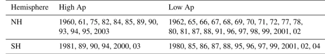
Table 1.Separation of data according to the Ap index. NH winters are referred to as 1961 for 1960/1961, etc.
Hemisphere High Ap Low Ap
NH 1960, 61, 75, 82, 84, 85, 89, 90, 1962, 65, 66, 67, 68, 69, 70, 71, 72, 77, 78, 93, 94, 95, 2003 80, 81, 87, 88, 91, 96, 97, 98, 99, 2001, 02
SH 1981, 89, 90, 94, 2000, 03 1980, 85, 86, 87, 88, 95, 96, 97, 99, 2001, 02, 04
3 Results and discussion
3.1 Transient simulation
A comprehensive simulation (hereafter denoted as S-TRANSIENT) covering the period 1960 to 2004 was carried out to study solar variability effects, including photolysis and heating rate variations using the high-resolution short-wave code FUBRad (Nissen et al., 2007), as well as particle pre-cipitation effects (Baumgaertner et al., 2010, 2009). The de-scription of the simulation and results concerning middle at-mosphere effects resulting from solar activity variations will be presented elsewhere.
The surface air temperature effect found by Sepp¨al¨a et al. (2009) triggered the present study, and an analogous analy-sis was therefore carried out in that the dataset was separated according to the yearly average wintertime Ap index, used as proxy for the overall geomagnetic activity level. The analy-sis is done separately for the Northern and Southern Hemi-sphere. The division into high and low geomagnetic activity years according to the Ap index is summarised in Table 1. The mean Ap value of 13.5 was used as a threshold for the high-low separation.
The NH temperature difference1T=High Ap−Low Ap for the winter season DFJ (December-January-February) is presented in Fig. 1 for the simulation results (left) and the reanalysis (right), taken from Sepp¨al¨a et al. (2009). There are some remarkable similarities between the temperature patterns found in the simulation and the ERA-40 reanaly-sis (Sepp¨al¨a et al., 2009, see their Figs. 2 and 3). Both the reanalysis data and the model show a negative anomaly of about 2 K over the North Atlantic, and a positive anomaly over the Arctic Sea, especially pronounced east of Green-land. The strongest warm anomaly is situated over Siberia in the reanalysis data, the model, however, shows this warm anomaly approximately centred around Svalbard. It should be noted that a perfect pattern match between the model and the reanalysis is not expected because the dynamics of the model were not relaxed to the observed meteorology. Hence, the synoptic situation in the model is different to the situation in the reanalysis at any given time. The model was however driven with observed sea surface temperatures (SST) and sea ice masks (HadISST1, see Rayner et al., 2003), which are expected to influence the SAT. Therefore, SST interannual variability can lead to aliasing effects in the SAT patterns
described above. The same years as used for the surface temperature calculation were used for Fig. 2 which shows the difference between the SSTs in years of high and low geomagnetic activity. The differences are generally smaller than 1 K and thus unlikely to alias the surface temperature result presented above. However, sensitivity simulations us-ing boundary conditions from a sus-ingle year are presented in the next section, completely eliminating the possibility of aliasing of SSTs and other influencing factors such as UV variability. Sepp¨al¨a et al. (2009) considered the influence of sudden stratospheric warmings (SSW) on their results, which lead them to exclude years with SSWs from the analysis (see their Fig. 3). This is not possible for the model results be-cause SSWs did not occur in the same years as in the reanal-ysis, and therefore different years would have to be excluded. Figure 3 depicts the SH temperature differences for the months JJA (June-July-August) for which Sepp¨al¨a et al. (2009) found the largest anomalies in the SH. Note that only years from 1979 onward were used here to be consistent with the study by Sepp¨al¨a et al. (2009). The model and reanaly-sis (Fig. 6 of Sepp¨al¨a et al., 2009) again show similar tem-perature patterns. The Antarctic peninsula is warmer by ap-proximately 2 K, and the area east of the Ross Sea is colder by up to 4 K. However, the model also shows a distinct cold anomaly in East Antarctica, which is absent in the reanalysis dataset. This might be due to the sparse measurement den-sity there, but could also be a result of the small number of years used for analysing the SH. In the following, we will mainly focus on the NH temperature pattern due to the larger number of years available for that region thus improving the statistics. Further problems associated with the SH pattern will be discussed in Sect. 3.2.
Fig. 1. Left: Northern Hemisphere DJF surface temperature difference between years of high and low geomagnetic activity (see Table 1). Left: transient simulation (S-TRANSIENT), right: from ERA-40 reanalysis data, taken from (Sepp¨al¨a et al., 2009, their Fig. 2). Red/blue colours indicate positive/negative differences.
Fig. 2. As Fig. 1 (left) but for sea surface temperatures from HadISST1 dataset as used in the simulation S-TRANSIENT.
in the “low” and “high” categories as in Table 1) and the ERA-40 data. From 100 different sets the mean correlation coefficient was found to be−0.01; ignoring the sign of each correlation coefficient yields a mean of 0.25. In the light of these findings the correlation coefficient of 0.35 warrants fur-ther analysis of the phenomenon.
In order to show that in the model the geomagnetic ac-tivity related NOxchanges in the polar stratosphere are not masked by dynamical influence, we calculated the corre-lation between the mean Ap index (November-December-January average) and the NOxmixing ratio at 45 km north of 70◦N (December-January-February average) which is shown in Fig. 4. The resulting correlation coefficient is 0.83. A similar result is obtained if only the years listed in Table 1
are used (denoted by red stars; correlation coefficient: 0.82). Thus, NOxenhancements produced by strong geomagnetic activity lead to significant enhancements in the upper strato-sphere, with only a weak dependence on other factors such as variable dynamical conditions that influence vertical or hori-zontal transport.
3.2 Sensitivity study: cyclic boundary conditions
In order to minimise possible aliasing effects of boundary conditions other than geomagnetic activity on the SAT, two additional nine-year simulations were carried out, one with high geomagnetic activity, and one with low geomagnetic activity. They are both based on the setup of the transient simulation described above, except that boundary conditions were taken from the year 2000 and repeated for every year of the simulation. These boundary conditions include:
1. sea surface temperatures and sea ice masks,
2. chemical tracers with a long lifetime, which are “nudged” towards observed values at the surface: green-house gases (CO2, N2O, CH4), ozone depleting sub-stances (CFCl3, CF2Cl2, CH3CCl3, CCl4, CH3Cl, CH3Br, CF2ClBr, CF3Br),
3. emissions of short-lived tracers: NO, CO, C2H4, C2H6, C4H10, CH3CHO, CH3COCH3, CH3COOH, CH3OH, HCHO, HCOOH, SO2, NH3, DMS, NOxfrom aircraft, 4. solar flux for photolysis and radiative heating, and the 5. geomagnetic activity (EPP-NOxinput).
Fig. 3. Southern Hemisphere JJA temperature difference (K) be-tween years of high and low geomagnetic activity (see Table 1) from the transient simulation. Red/blue colours indicate positive/negative differences.
after the applied shift of one month to account for down-ward transport not captured by the model, was 25.2. For the first simulation, hereafter termed S-EPP, the SPACENOX submodel providing the EPP-NOxinput at the upper bound-ary, was switched on. For the second simulation the sub-model was turned off, effectively corresponding to years of very low geomagnetic activity, where no NOxfrom the EPP source reaches the mesosphere. This simulation is hereafter referred to as S-noEPP.
It should be noted that cyclic boundary conditions will in-troduce discontinuities from December to January since they are not taken from consecutive years but rather from the same year. However, the seasonal cycle is strong for SSTs as it is for chemical boundary conditions, therefore this issue is not regarded as problematic.
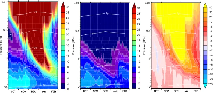
By subtracting the results of the simulation S-noEPP from the simulation S-EPP (i.e. S-EPP−S-noEPP) the influence of EPP-NOx can be extracted. Since the model is free-running, there is also inherent variability, which effectively adds noise to the results. Moreover, as has been pointed out by Sepp¨al¨a et al. (2009), care has to be taken regarding years with SSWs, which are the strongest manifestation of strato-spheric interannual variability. Both simulations were run for nine years, giving a total of 18 NH winters. Fig. 6 shows the NOxmixing ratios for the simulations S-EPP (left) and S-noEPP (middle) as well as the difference (right) for an exemplary NH winter. Large confined NOxenhancements are evident that propagate downwards during the course of the winter as expected. The colour scale has been chosen to ease comparison with Fig. 2 (top) of Sepp¨al¨a et al. (2007b), who showed NO2mixing ratios from GOMOS satellite mea-surements for the same latitude region. Since the Ap index for simulation S-EPP originates from the year 2003, the NH winter 2003/2004 is best suited for a direct comparison. In
Fig. 4.Ap index versus NOxmixing ratios (nmol mol−1) at 45 km altitude for Northern Hemisphere winters, from the transient simu-lation. Black crosses: all available years, red stars: selected years according to Table 1.
Fig. 5. Southern Hemisphere JJA surface temperature difference (K),1T =TS−EPP−TS−noEPP. Red/blue colours indicate posi-tive/negative differences.
the simulation NOx enhancements reach 35 km at the end of December, very similar to the NO2enhancements found by GOMOS. Note that in December/January an SSW oc-curred, which is not reproduced by the model in this partic-ular year of the model simulation. Consequently, GOMOS observed a sudden drop in NO2mixing ratios during this pe-riod, whereas high NOxmixing ratios persist in the simula-tion.
Fig. 6.Left: zonal mean NOxmixing ratios (nmol mol−1) from simulation S-EPP for an exemplary Northern Hemisphere winter poleward of 60◦N. Middle: as left panel, but from simulation S-noEPP. Right: mixing ratio difference NOS−EPPx −NOS−noEPPx . Red-yellow/blue colours indicate positive/negative differences. The white contour lines denote the altitude in km in all panels.
Fig. 7. NH DJF surface temperature difference1T =TS−EPP−TS−noEPP. Left: all years, right: only years without SSWs. Red/blue colours indicate positive/negative differences.
significance level, calculated using the Student’s t-test. For geophysical applications, the number of independent points for the test is not a priori equal to the number of data points. From a physical perspective, there is no evidence that con-ditions in any given year should be the major driver for the polar surface temperatures in the subsequent winter. There-fore, we argue that polar surface temperatures are probably independent and have thus used the number of data points, i.e. years, for the test formula. Also note that the trends of the timeseries (not shown) in this region are negligible as expected.
shows the same dataset but SSW years excluded, which can be directly compared to Sepp¨al¨a et al. (2009) Fig. 3. As in the reanalysis study, the pattern becomes more pronounced, the cooling in the Eastern North Atlantic is now stronger, al-though it still does not cover Greenland, in contrast to the reanalysis results. Also, the United States SAT now shows a consistent warming.
Results for the SH winter months JJA are depicted in Fig. 5. Similar to the transient simulation and the reanal-ysis (Fig. 3 and Sepp¨al¨a et al., 2009, their Fig. 6), negative anomalies of up to 2 K are found around the Ross Sea and the western side of the Antarctic Peninsula, positive anomalies of 2 K are found on and north of the Antarctic Peninsula. The large negative anomaly in East Antarctica seen in Fig. 3 is not present in this set of simulations. The 95 % significance level from a Student’s t-test (see above) is indicated by the white contours. Note that the main features of the pattern are not significant. Using different subsets of the simulation (not shown), unlike the NH behaviour, very different patterns are obtained. Possible reasons for this behaviour are discussed in the next section. However, as already pointed out above, we focus the presented analysis on the NH because of the low significance of the SH response.
The differences in the temperature patterns in Fig. 7 (Fig. 5) compared with Fig. 1 (Fig. 3) are potentially due to the use of extreme levels of strong and weak geomag-netic activity in the sensitivity study, compared with those in the transient simulation. The overall similarity of the tem-perature patterns in the reanalysis, transient simulation, and sensitivity simulations suggest that the coupling mechanism linking geomagnetic activity and surface temperature is op-erating in the EMAC model. The precise pattern is sensitive to the absolute levels of the geomagnetic activity. However, substantial differences between the transient and sensitivity temperature patterns occur.
3.3 Linking EPP-NOxand SAT anomalies
As shown by Baumgaertner et al. (2009), geomagnetic activ-ity related polar winter NOx enhancements leads to strato-spheric ozone loss due to the catalytic destruction of odd oxygen. Therefore, ozone mixing ratios are expected to be significantly different between the simulations S-EPP and S-noEPP. Ozone differences between these two simulations (1O3=OS3−EPP−OS3−noEPP) as a function of latitude and al-titude for DJF are shown in Fig. 8.
Indeed, stratospheric ozone is reduced by up to 1 µmol mol−1in the middle and upper stratosphere (approxi-mately 20 % in the upper stratosphere, 10 % at 20 hPa) in the polar area. This leads to a mean total column ozone loss of up to 35 DU. Since ozone is an important radiatively active gas, in general stratospheric ozone concentration changes lead to effects in temperatures. During polar winter, the affected re-gion is mostly dark, so effects caused by the absorption of solar short-wave radiation are expected to be small.
How-Fig. 8.Climatological DJF change (µmol mol−1) of ozone,1O3= OS−EPP3 −OS−noEPP3 . Red-yellow/blue colours indicate posi-tive/negative differences.
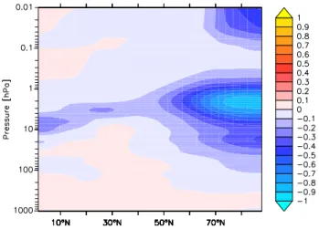
ever, ozone is also a radiative coolant, an effective green-house gas, and it absorbs longwave radiation from the sur-face. Ozone changes can therefore potentially lead to temper-atures changes even during the polar night. Ozone depletion effects on temperature and dynamics have been subject to in-tensive research in the past (Christiansen et al., 1997; Randel and Wu, 1999; Austin et al., 2001; Langematz et al., 2003; Shine et al., 2003, and others), mainly focusing on CFC in-duced ozone depletion. In general, such responses have been shown to be dependent on latitude, season, and on the vertical profile of ozone loss. For the analysis here, a relevant study was conducted by Langematz et al. (2003). Using sensitivity simulations with prescribed ozone loss and a control simu-lation, they found a heating above the stratopause and cool-ing below for the NH polar winter (see their Fig. 8a). Uscool-ing additional radiative transfer calculations, which show only a warming throughout the stratosphere (their Fig. 9), they con-cluded that the decrease in ozone radiative cooling is respon-sible for the warming in the simulation with ozone depletion. The cooling below the stratopause was attributed to dynam-ical heating induced by a decrease of the mean meridional circulation. Figure 9 presents the temperature differences be-tween the two sensitivity simulations performed here. The figure shows that polar lower stratospheric temperatures be-tween 200–5 hPa decrease by up to 4 K in the S-EPP sim-ulation, and above 4 hPa polar temperatures increase in the S-EPP simulation, indicating that the two-fold response de-scribed by Langematz et al. (2003) is likely to be also respon-sible for the effects observed in the EMAC simulations.
Fig. 9. Climatological DJF change of temperature (K), 1T =
TS−EPP−TS−noEPP. Red-yellow/blue colours indicate posi-tive/negative differences.
vortex. We calculated the NAM index for the model results from the geopotential heights using the zonal mean EOF (empirical orthogonal function) method described by Bald-win and Thompson (2009). The change in the polar (60◦N– 90◦N) zonal mean geopotential height anomalies between the two simulations are presented in Fig. 10. The figure shows how a strong negative anomaly which first develops early in the winter season at higher altitudes and descends downwards reaching the mid-stratosphere by February. Us-ing the model geopotential heights, the NAM index was cal-culated and histograms of the NAM indices between 10 hPa and the tropopause for DJF are shown in Fig. 11. The solid (dashed) black line is the histogram for the simulation S-EPP (S-noEPP). While the tails of the distribution are similar, the probability for NAM indices within the range±2 is different between the two simulations: positive NAM indices are more likely in the S-EPP simulation, thus indicating a stronger Arctic polar vortex in the S-EPP simulation. The error bars show the standard deviations resulting from the individual years, indicating that the result is robust. It was investigated if the occurence of SSWs in some of the simulated years (four in S-noEPP and three in S-EEP) impacts these results by doing the histogram analysis only for the years where no SSWs occurred. The results are shown as the solid (dashed) grey lines for the S-EPP (S-noEPP) simulation. Qualitatively the result does not change, again highlighting the robustness of the result.
From Baldwin and Dunkerton (2001) and others it is known that anomalous weather regimes characterised by NAM index anomalies can propagate down into the tropo-sphere. This is also observed in the simulations presented here, as shown in Fig. 12, where we show a single exem-plary winter from both simulations (top: EPP, bottom: S-noEPP). For example, in this case in the S-EPP simulation a positive NAM anomaly develops in the stratosphere in late
Fig. 10. Climatological change of geopotential height anomalies (normalised at every level with respect to standard deviation) for the region 60◦N–90◦N,1Z=ZS−EPP−ZS−noEPP. Red-yellow/blue colours indicate positive/negative differences.
−3 −2 −1 0 1 2 3
NAM index
Fig. 11. NAM index histogram for the altitude region 10 hPa– 200 hPa for DJF. Solid black: S-EPP, dashed black: S-noEPP. The error bars show the standard deviation calculated from the individ-ual years. The grey lines show the analogous results for only those years where no SSWs occurred.
December, reaching the surface by mid-January. This is not observed in the equivalent S-noEPP simulation.
Fig. 12. NAM index for an exemplary winter calculated from simulation S-EPP (top) and S-noEPP (bottom). Red-yellow/blue colours indicate positive/negative differences.
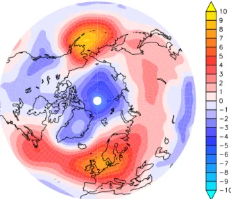
Fig. 13. DJF surface pressure difference (hPa) 1p=pS−EPP−
pS−noEPP, SSW years excluded. Red-yellow/blue colours indicate positive/negative differences.
observed temperature patterns found in the SAT difference between S-EPP and S-noEPP (Fig. 7). The NAM phase can also be detected in the surface pressure. The positive phase is characterised by anomalously low pressures at high lat-itudes and higher than average pressures at mid-latlat-itudes. Figure 13 depicts the DJF surface pressure differences
be-tween the simulations S-EPP and S-noEPP. The negative pressure anomalies over Greenland and positive anomalies at mid-latitudes indicate a positive NAM phase as expected, although the low pressure region does not extend over Scan-dinavia as the NAM often does. Since the NAM related NAO (see e.g. Hurrell and Kushnir, 2003) index is often calculated as the pressure difference between the Azores and Reykjavik, Iceland, the predicted pattern also influences the NAO index. In the light of this mechanism, a possible reason for the lack of a similarly significant response in the SH could be the fact that the SH polar vortex is already much colder and more stable than in the NH. This potentially makes it less suscep-tible to perturbations by NOxenhancements. However, the SH response is subject to further work.
4 Conclusions
where the boundary conditions were repeated on a yearly ba-sis. The only difference between the two simulations was that geomagnetic activity related NOx production was switched on in one simulation, thus allowing us to identify purely NOx induced effects. Again, similar surface temperature patterns were found. This indicates that these patterns are indeed re-lated to NOx production due to geomagnetic activity. The following mechanism was hypothesised from the model re-sults: The geomagnetic activity/Energetic Particle Precipi-tation related NOx production leads to ozone depletion in the stratosphere. Changes in the radiative budget and sub-sequently of the mean meridional circulation cool the lower stratosphere and strengthen the polar vortex. Associated pos-itive NAM anomalies propagate into the troposphere, where typical positive NAM surface pressure and temperature pat-terns occur. Therefore, enhanced geomagnetic activity and NOx production appear to trigger positive NAM phases at the surface level in the model. Further studies are required to confirm these results and the proposed mechanism as the findings indicate a stronger link of surface climate to space weather than has previously been assumed.
Supplementary material related to this article is available online at:
http://www.atmos-chem-phys.net/11/4521/2011/ acp-11-4521-2011-supplement.pdf.
Acknowledgements. This research was funded by the TIES project within the DFG SPP 1176 CAWSES. Thanks go to all MESSy developers and users for their support. We thank Cora Randall and Dan Marsh, and Robert Hibbins for fruitful discussions. The model simulations were performed on the POWER-6 computer at the RZG and DKRZ. The Ferret program (http://www.ferret.noaa.gov) from NOAA’s Pacific Marine Environmental Laboratory was used for creating some of the graphics in this paper. The work of AS was funded through the FP7-PEOPLE-IEF Marie Curie project EPPIC/237461.
The service charges for this open access publication have been covered by the Max Planck Society.
Edited by: W. Lahoz
References
Austin, J., Langematz, U., Dameris, M., Pawson, S., Pitari, G., Shine, K. P., and Stordal, F.: Stratospheric ozone and its links to climate change, pp. 191–222, Office for Off. Publ. of the Eur. Comm., Luxembourg, 2001.
Austin, J., Tourpali, K., Rozanov, E., Akiyoshi, H., Bekki, S., Bodeker, G., Br¨uhl, C., Butchart, N., Chipperfield, M., Deushi, M., Fomichev, V. I., Giorgetta, M. A., Gray, L., Kodera, K., Lott, F., Manzini, E., Marsh, D., Matthes, K., Nagashima, T., Shibata, K., Stolarski, R. S., Struthers, H., and Tian, W.:
Coupled chemistry climate model simulations of the solar cy-cle in ozone and temperature, J. Geophys. Res., 113, D11306, doi:10.1029/2007JD009391, 2008.
Baldwin, M. P. and Dunkerton, T. J.: Stratospheric harbingers of anomalous weather regimes, Science, 294, 581–584, doi:10.1126/science.1063315, 2001.
Baldwin, M. P. and Thompson, D. W. J.: A critical comparison of stratosphere-troposphere coupling indices, Q. J. Roy. Meteorol. Soc., 135, 1661–1672, doi:10.1002/qj.479, 2009.
Baumgaertner, A. J. G., J¨ockel, P., and Br¨uhl, C.: Energetic particle precipitation in ECHAM5/MESSy1 – Part 1: Downward trans-port of upper atmospheric NOxproduced by low energy elec-trons, Atmos. Chem. Phys., 9, 2729–2740, doi:10.5194/acp-9-2729-2009, 2009.
Baumgaertner, A. J. G., J¨ockel, P., Riede, H., Stiller, G., and Funke, B.: Energetic particle precipitation in ECHAM5/MESSy – Part 2: Solar proton events, Atmos. Chem. Phys., 10, 7285–7302, doi:10.5194/acp-10-7285-2010, 2010.
Boberg, F. and Lundstedt, H.: Solar Wind Variations Re-lated to Fluctuations of the North Atlantic Oscillation, Geo-phys. Res. Lett., 29, 1718, doi:10.1029/2002GL014903, 2002. Br¨uhl, C., Steil, B., Stiller, G., Funke, B., and J¨ockel, P.:
Nitrogen compounds and ozone in the stratosphere: com-parison of MIPAS satellite data with the chemistry climate model ECHAM5/MESSy1, Atmos. Chem. Phys., 7, 5585–5598, doi:10.5194/acp-7-5585-2007, 2007.
Christiansen, B., Guldberg, A., Hansen, A. W., and Riishøjgaard, L. P.: On the response of a three-dimensional general circula-tion model to imposed changes in the ozone distribucircula-tion, J. Geo-phys. Res., 102, 13051–13078, doi:10.1029/97JD00529, 1997. Clilverd, M. A., Rodger, C. J., and Ulich, T.: The
impor-tance of atmospheric precipitation in storm-time relativistic electron flux drop outs, Geophys. Res. Lett., 33, L01102, doi:10.1029/2005GL024661, 2006.
Funke, B., L´opez-Puertas, M., Gil-L´opez, S., von Clarmann, T., Stiller, G. P., Fischer, H., and Kellmann, S.: Down-ward transport of upper atmospheric NOxinto the polar strato-sphere and lower mesostrato-sphere during the Antarctic 2003 and Arctic 2002/2003 winters, J. Geophys. Res., 110, D24308, doi:10.1029/2005JD006463, 2005.
Gruzdev, A. N., Schmidt, H., and Brasseur, G. P.: The effect of the solar rotational irradiance variation on the middle and upper at-mosphere calculated by a three-dimensional chemistry-climate model, Atmos. Chem. Phys., 9, 595–614, doi:10.5194/acp-9-595-2009, 2009.
Hood, L. L. and Soukharev, B. E.: Solar induced variations of odd nitrogen: Multiple regression analysis of UARS HALOE data, Geophys. Res. Lett., 33, L22805, doi:10.1029/2006GL028122, 2006.
Hurrell, J. W., Kushnir, Y., Ottersen, G., and Visbeck, M. (Eds.): An Overview of the North Atlantic Oscillation, in: The North Atlantic Oscillation, 134, doi:10.1029/134GM01, Geophys. Monog. Ser., AGU, Washington DC, 2003.
IPCC: IPCC Fourth Assessment Report: Climate Change 2007, Cambridge University Press, Cambridge, 2007.
model ECHAM5/MESSy1: consistent simulation of ozone from the surface to the mesosphere, Atmos. Chem. Phys., 6, 5067– 5104, doi:10.5194/acp-6-5067-2006, 2006.
J¨ockel, P., Kerkweg, A., Pozzer, A., Sander, R., Tost, H., Riede, H., Baumgaertner, A., Gromov, S., and Kern, B.: Development cycle 2 of the Modular Earth Submodel System (MESSy2), Geosci. Model Dev. Discuss., 3, 1423–1501, doi:10.5194/gmdd-3-1423-2010, 2010.
Langematz, U., Kunze, M., Kr¨uger, K., Labitzke, K., and Roff, G. L.: Thermal and dynamical changes of the stratosphere since 1979 and their link to ozone and CO2changes, J. Geophys. Res., 108, 4027, doi:10.1029/2002JD002069, 2003.
Lelieveld, J., Br¨uhl, C., J¨ockel, P., Steil, B., Crutzen, P. J., Fis-cher, H., Giorgetta, M. A., Hoor, P., Lawrence, M. G., Sausen, R., and Tost, H.: Stratospheric dryness: model simulations and satellite observations, Atmos. Chem. Phys., 7, 1313–1332, doi:10.5194/acp-7-1313-2007, 2007.
Lu, H., Clilverd, M. A., Sepp¨al¨a, A., and Hood, L. L.: Geomagnetic perturbations on stratospheric circulation in late winter and spring, J. Geophys. Res., 113, D16106, doi:10.1029/2007JD008915, 2008.
Mayaud, P. N.: Derivation, Meaning, and Use of Geomagnetic In-dices, Geophysical Monograph 22, Am. Geophys. Union, Wash-ington DC, USA, 1980.
Meehl, G. A., Arblaster, J. M., Matthes, K., Sassi, F., and van Loon, H.: Amplifying the Pacific climate system response to a small 11 year solar cycle forcing, Science, 325, 1114–1118, 2009. Nissen, K. M., Matthes, K., Langematz, U., and Mayer, B.: Towards
a better representation of the solar cycle in general circulation models, Atmos. Chem. Phys., 7, 5391–5400, doi:10.5194/acp-7-5391-2007, 2007.
Randall, C. E., Harvey, V. L., Manney, G. L., Orsolini, Y., Co-drescu, M., Sioris, C., Brohede, S., Haley, C. S., Gordley, L. L., Zawodny, J. M., and Russell, J. M.: Stratospheric effects of en-ergetic particle precipitation in 2003–2004, Geophys. Res. Lett., 32, L05802, doi:10.1029/2004GL022003, 2005.
Randall, C. E., Harvey, V. L., Singleton, C. S., Bailey, S. M., Bernath, P. F., Codrescu, M., Nakajima, H., and Russell, J. M.: Energetic particle precipitation effects on the Southern Hemisphere stratosphere in 1992–2005, J. Geophys. Res., 112, D08308, doi:10.1029/2006JD007696, 2007.
Randel, W. J. and Wu, F.: Cooling of the Arctic and Antarctic polar stratospheres due to ozone depletion., J. Climate, 12, 1467–1479, doi:10.1175/1520-0442(1999)012¡1467:COTAAA¿2.0.CO;2, 1999.
Rayner, N. A., Parker, D. E., Horton, E. B., Folland, C. K., Alexan-der, L. V., Rowell, D. P., Kent, E. C., and Kaplan, A.: Global analyses of sea surface temperature, sea ice, and night marine air temperature since the late nineteenth century, J. Geophys. Res., 108(D14), 4407, doi:10.1029/2002JD002670, 2003.
Roeckner, E., Brokopf, R., Esch, M., Giorgetta, M., Hagemann, S., Kornblueh, L., Manzini, E., Schlese, U., and Schulzweida, U.: Sensitivity of simulated climate to horizontal and vertical resolution in the ECHAM5 atmosphere model, J. Climate, 19, 3771, doi:10.1175/JCLI3824.1, 2006.
Rozanov, E., Callis, L., Schlesinger, M., Yang, F., Andronova, N., and Zubov, V.: Atmospheric response to NOysource due to en-ergetic electron precipitation, Geophys. Res. Lett., 32, L14811, doi:10.1029/2005GL023041, 2005.
Sander, R., Kerkweg, A., J¨ockel, P., and Lelieveld, J.: Technical note: The new comprehensive atmospheric chemistry module MECCA, Atmos. Chem. Phys., 5, 445–450, doi:10.5194/acp-5-445-2005, 2005.
Sepp¨al¨a, A., Clilverd, M. A., and Rodger, C. J.: NOxenhancements in the middle atmosphere during 2003–2004 polar winter: Rela-tive significance of solar proton events and the aurora as a source, J. Geophys. Res., 112, D23303, doi:10.1029/2006JD008326, 2007a.
Sepp¨al¨a, A., Verronen, P. T., Clilverd, M. A., Randall, C. E., Tamminen, J., Sofieva, V., Backman, L., and Kyr¨ol¨a, E.: Arc-tic and AntarcArc-tic polar winter NOx and energetic particle pre-cipitation in 2002-2006, Geophys. Res. Lett., 34, L12810, doi:10.1029/2007GL029733, 2007b.
Sepp¨al¨a, A., Randall, C. E., Clilverd, M. A., Rozanov, E., and Rodger, C. J.: Geomagnetic activity and polar surface air temperature variability, J. Geophys. Res., 114, A10312, doi:10.1029/2008JA014029, 2009.
Siskind, D. E., Nedoluha, G. E., Randall, C. E., Fromm, M., and Russell III, J. M.: An assessment of Southern Hemi-sphere stratospheric NOxenhancements due to transport from the upper atmosphere, Geophys. Res. Lett., 27, 329–332, doi:10.1029/1999GL010940, 2000.
Shine, K. P., Bourqui, M. S., Forster, P. M. D. F., Hare, S. H. E., Langematz, U., Braesicke, P., Grewe, V., Ponater, M., Schnadt, C., Smith, C. A., Haigh, J. D., Austin, J., Butchart, N., Shindell, D. T., Randel, W. J., Nagashima, T., Portmann, R. W., Solomon, S., Seidel, D. J., Lanzante, J., Klein, S., Ramaswamy, V., and Schwarzkopf, M. D.: A comparison of model-simulated trends in stratospheric temperatures, Q. J. Roy. Meteorol. Soc., 129, 1565– 1588, doi:10.1256/qj.02.186, 2003.
Thejll, P., Christiansen, B., and Gleisner, H.: On correlations between the North Atlantic Oscillation, geopotential heights, and geomagnetic activity, Geophys. Res. Lett., 30, 1347, doi:10.1029/2002GL016598, 2003.