AN EFFICIENT NON-LINEAR GBT-BASED FINITE ELEMENT FOR STEEL-CONCRETE BEAMS

Lisbon, Portugal, July 22-24, 2015

AN EFFICIENT NON-LINEAR GBT-BASED FINITE ELEMENT FOR

STEEL-CONCRETE BEAMS

D. Henriques*, R. Gonçalves** and D. Camotim***

* Faculdade de Ciências e Tecnologia, Universidade Nova de Lisboa 2829-516 Caparica, Portugal ** CEris, ICIST and Departamento de Engenharia Civil, Faculdade de Ciências e Tecnologia

Universidade Nova de Lisboa 2829-516 Caparica, Portugal e-mail: [email protected]

***CEris, ICIST, DECivil, Instituto Superior Técnico, Universidade de Lisboa, 1049-001 Lisbon, Portugal e-mail: [email protected]

Keywords: Steel-concrete composite beams; Generalized Beam Theory (GBT); Shear Lag; Non-linear behaviour.

Abstract. A computationally efficient GBT-based beam finite element is presented, specifically developed for capturing the materially non-linear behaviour of wide-flange steel-concrete composite beams. The element incorporates shear lag effects, as well as concrete and steel non-linear material behaviour. Analytical solutions for elastic shear lag problems are derived and a set of materially linear and non-linear numerical examples is presented, showing that the proposed beam finite element captures accurately all relevant phenomena with a very small computational cost. For validation and comparison purposes, results obtained with shell/brick finite element models are also presented. 1 INTRODUCTION

The Generalized Beam Theory (GBT) is a thin-walled prismatic bar theory that efficiently handles cross-section in-plane and out-of-plane (warping) deformation, through the inclusion of “cross-section deformation modes”. GBT was introduced by R. Schardt almost 50 years ago [1,2] and it has since been continuously and considerably developed. Presently, it is rather well established as a very efficient and valuable tool for analysing prismatic thin-walled beams — see, e.g., [3-6].

In the field of steel-concrete composite bridge first-order/free vibration/buckling analyses, very promising results have been obtained with GBT [7], due to its straightforward capability of including relevant phenomena such as shear lag and shear connection flexibility. In particular, it was shown that GBT (i) leads to accurate solutions with a small number of deformation modes (and thus a small number of DOFs) and (ii) makes it possible to acquire a valuable insight into the mechanics of the problem addressed through the modal decomposition of the solution.

The proposed beam finite element is developed by making an appropriate trade-off between accuracy and computational efficiency, aiming at simplicity (a key goal). In particular, (i) membrane shear deformation is only allowed in wide flanges (to capture shear lag effects) and in the steel girder web (to capture vertical shear effects) and (ii) the stresses and strains are constrained in order to make it possible to reduce the number of deformation modes necessary to achieve accurate results and also to employ simple material models for both concrete and steel.

The outline of the paper is as follows. Section 2 presents the fundamental aspects of the beam finite element. Section 3 discusses a set of application examples, which include both analytical and numerical solutions. For comparison and validation purposes, results obtained with shell and brick finite element models, using ADINA [8] and ATENA [9], respectively, are also presented. The paper closes in Section 4, with the concluding remarks.

2 FINITE ELEMENT FORMULATION

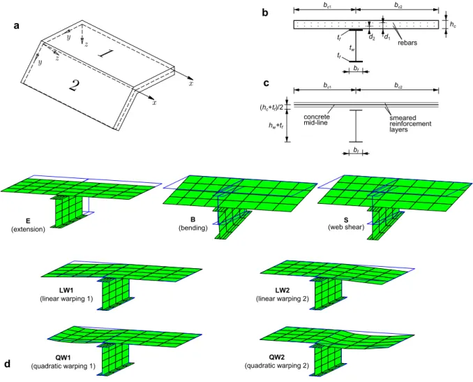
The physically non-linear beam finite element is based on the general formulation presented in [10,11], discarding geometric non-linear effects and including additional modifications/simplifications pertaining to the particular problem being addressed. With the Kirchhoff thin plate assumption and the wall mid-surface local axes shown in Fig. 1(a), the displacement vector for each wall, U, is expressed as





U y y (2)

where the commas indicate differentiations, (x) is a column vector collecting the mode amplitude functions and u(y),v(y),w(y) are column vectors containing the displacement functions of the wall mid-line along x, y, z, respectively, for each deformation mode, which may be determined from the procedures outlined in [12,13]. The non-null small strain components are grouped in vector t = [xx yy xy], which is subdivided into membrane (M)

and bending (B) components, reading





In general, a plane stress state is assumed in each wall and the non-null components are grouped in vector t = [xx yy xy], which is related to  through the particular constitutive

law adopted. Within a Newton-Raphson iterative solution, the tangent stress-strain relation is written as d = Ct d, where Ct is the consistent tangent constitutive matrix pertaining to the

Figure 1: (a) Thin-walled member local coordinate systems; steel-concrete composite beam cross-section (b) geometry, (c) wall mid-lines and reinforcement layers, and (d) cross-section deformation modes.

The out-of-balance force vector g, the tangent stiffness matrix Kt and the incremental load

vector f are obtained from

, , , , , , , , , , ,









g   

(4)

where qare forces acting along the walls mid-surface  (for simplicity, volume forces are not considered).

For the strains, the following additional assumptions are introduced: (i) the cross-section is

in-plane undeformable (   xyB 0

B yy M

yy  

 , which also eliminates torsion) and (ii) Vlasov’s

null membrane shear strain assumption (_xyM 0) is enforced in compact walls (typically, the narrow steel flanges of the I-section). These assumptions reduce the number of admissible cross-section deformation modes to those shown in Fig. 1(d): (E) axial extension, (B) Euler-Bernoulli bending assuming uncracked concrete, (S) uniform web shearing and (LW/QW) linear/quadratic shear lag warping modes in each concrete flange. The E mode must be included in the analyses even if no axial force is being applied, in order to capture the shift of the neutral line caused by cracking and/or shear lag. Although additional shear deformation modes in the steel web and/or concrete slab can be straightforwardly added, using e.g. sinusoidal warping functions [7,12], the examples presented in Section 3 show that there is no significant gain in considering more than the LW/QW modes.

With the interpolation functions adopted, the proposed beam finite element involves 8 DOFs for the B + S modes (2 DOFs for each element end node and mode) plus 3 DOFs for each warping mode (1 DOF for each end node and 1 DOF for an intermediate node), leading to a total of only 23 DOFs if all 7 deformation modes of Fig. 1(d) are included in the analysis. For symmetric flanges, the shear lag modes may be paired (i.e., LW1+LW2 and QW1+QW2), leading to a reduced 17 DOF element.

For the stresses, the only non-null stress components are B xx M xx 

 , and M

xy

 , except where

Vlasov’s assumption is enforced, in which case _xyM 0 and an uniaxial stress state is obtained (xx  0). As in [10,11], a small-strain elastic-perfectly plastic material law is

employed for steel, with the St. Venant-Kirchhoff law for the elastic part, the von Mises yield function and associated flow rule. The stresses at the end of each iteration are calculated using the backward Euler return algorithm under the yy = 0 assumption and Ct corresponds to the

associated (consistent) tangent constitutive matrix. The relevant material parameters are Young’s modulus E, the shear modulus G and the uniaxial yield stress fy. The subscripts s and

a are employed to designate rebars and steel, respectively.

For concrete, zero tensile strength is assumed and a smeared fixed crack-type approach is followed. Together with a plane stress state under the yy = 0 constraint, this material model

implies that generalised cracking occurs at the onset of loading (along y at intermediate supports, at 45º near contraflexure zones and along x near maximum sagging bending zones). For both efficiency and simplicity, separate constitutive laws are adopted for xx and xy. The

longitudinal normal stresses are related to xx through an uniaxial law, without tensile strength

and a non-linear compressive branch up to the peak stress. It is assumed that unloading/reloading is elastic. In the examples presented in Section 3, the Eurocode 2 [14] relation for mean values is adopted for the ascending branch, which reads (all values are deemed positive) , 05 . 1 , , ) 2 ( 1 1 1 2 c c c c xx c xx f E k k k f               (5)

where c1 is the strain at the concrete peak stress fc. After the peak, a linear softening branch is

adopted down to zero stress, which is attained at a mesh adjusted “final” strain f, to mitigate

mesh sensitivity problems, reading

, 1 L d E f c c c

f   

where L is the finite element length and d is a material parameter which needs to be calibrated. A similar strategy for the post-peak response is implemented in ATENA. This uniaxial law is schematically given in Fig. 2(a). For the shear stresses, the non-linear elastic law depicted in Fig. 2(b) is adopted, where c is the maximum stress, Gc = Ec/2(1+c) is the

elastic shear modulus, c is Poisson’s ratio, and   1 is a reduction factor for cracked

concrete, which is somewhat similar to the shear retention factor employed in standard fixed smeared crack approaches.

Numerical integration is performed using Gauss quadrature, with 3 points along x, as in [11], and an arbitrary number of points along y and z in each wall. The load-displacement path is calculated using a standard incremental-iterative scheme with displacement control. The finite element procedure was implemented in MATLAB [15].

Figure 2: Stress-strain laws for concrete: (a) normal stresses and (b) shear stresses.

3 APPLICATIONS AND ILLUSTRATIVE EXAMPLES 3.1 Elastic shear lag

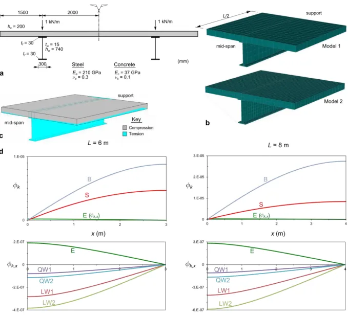
The first example concerns an elastic shear lag problem. Two simply supported wide flange steel-concrete twin-girder beams are analysed, with span lengths equal to L = 6.0, 8.0 m and the cross-section geometry and material parameters given in Fig. 3(a). The beams are subjected to 1 kN/m uniformly distributed vertical loads acting in the plane of the steel webs. Due to the problem double symmetry, only a quarter of the twin-beams is modelled (half of the length and cross-section). Note that the span-to-slab width ratio in this particular example is rather small, which constitutes a challenge for beam-type finite elements.

The GBT analyses are carried out with the 7 deformation modes of Fig. 1(d) and 8 equal length finite elements, which amounts to a total of 112 DOFs (after elimination of the constrained DOFs due to boundary conditions). Since an elastic behaviour is assumed, numerical integration is carried out with only 2 Gauss points along the thickness and 3 Gauss points along y, in each wall.

Figure 3: Elastic shear lag problem: (a) cross-section geometry, loading and material parameters, (b) brick element models, (c) neutral surface obtained with the brick model and (d) GBT mode amplitude functions.

The graphs in Fig. 3(d) plot the GBT individual mode amplitude functions (recall that, with (1)-(2), the amplitude functions for the modes with warping only are given by k,x rather than

by k) for 0  x  L/2, leading to the following conclusions:

(i) These are bending-dominated problems, as the B mode has the highest participation (maximum at mid-span, null at the supports). The influence of web shear deformation is revealed by the S mode which, naturally, has a higher participation for the shorter span (note however that web shearing is proportional to k,x, which is maximum at the

supports and null at mid-span).

(ii) The warping modes (E, LW, QW) have significantly lower participations, with the LW modes being the most relevant, followed by the E mode. Since these modes are related to the occurrence of shear deformation, their amplitude functions k,x are

approximate) shear lag warping mode and further reduce the number of modes (DOFs) included in the analyses. This issue will be further addressed in Sections 3.2 and 3.4.

(iii) The participations of the shear lag modes for the wider concrete flange (LW2 and QW2) are higher than their narrower flange counterparts (LW1 and QW1), which is due to the cross-section asymmetry and is in accordance with the stress distributions shown next.

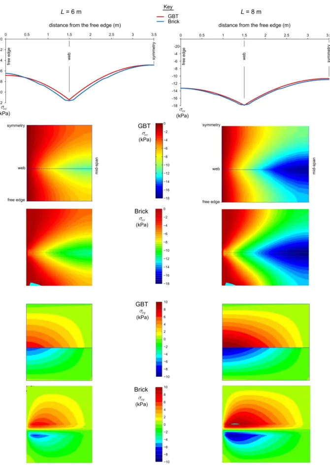
Fig. 4 compares the concrete slab mid-surface stresses obtained with GBT and the brick element models. The top graphs plot the mid-span xx distributions and the bottom figures

show surface plots of both xx and xy. The shear lag effects are clearly visible in the xx

distributions and, naturally, (i) the effect is more pronounced for the shorter span and (ii) the unequal concrete flange widths produce asymmetric stress distributions. In general, the GBT and brick model stresses (namely the mid-span values) are in very good agreement. This is rather remarkable given that the GBT elements have only a few deformation modes and that the neutral surface is very near the slab mid-surface, as shown in Fig. 3(c). GBT analyses were also carried out using sinusoidal warping modes (instead of the QW modes), with 1 to 4 half-waves in each concrete flange, but virtually identical results were obtained and therefore they are not shown.

Concerning the particular case of the mid-span stress graphs, an excellent agreement is observed. However, the GBT results predict a sharp peak over the web, whereas the brick models show a smooth transition due to the fact that the contact surface between the steel flange and concrete is modelled explicitly in this case. Note that the xy distributions over the

web show the same effect, as the GBT/brick results vary abruptly/smoothly from one side to the other. Concerning the xx surface plots, although the colour maps for each model do not

match exactly, a very good agreement is observed. Nevertheless, near the support, the brick models predict a higher shear lag effect. The xy surface plots provide evidence of this

mismatch, as the GBT solutions yield non-null shear stresses at x = 0. This effect can only be mitigated by including transverse extension modes in the analyses, but this renders the GBT formulation considerably more complex, particularly at the constitutive modelling level.

3.2 Analytical solutions for elastic shear lag

In particular cases, the GBT approach makes it possible to retrieve semi-analytical (or even analytical) solutions that provide in-depth information concerning the mechanics of the problem. For simply supported members subjected to sinusoidal transverse loads of the form

) / sin( x L q

q  , where q is the load amplitude, the exact solutions are _k _ksin(x/L), where the mode amplitudes _kconstitute the only unknowns and thus the DOF number equals the number of deformation modes. In the present formulation, with q= 1 kN/m vertical loads acting in the plane of the web and the 7 deformation modes shown in Fig. 1(d), due to the particular constraints adopted for the stress and strain fields, the GBT semi-analytical solution is reduced to

, 7 1 1 2 4 7 1                                            q q L L 

  C  D

  (7) , ) )( ( ,

12 , ,

3





ij ww dy Gt u v u v dy

Figure 4: Elastic shear lag problem: (a) mid-span xx distributions at the concrete slab height and (b) slab

where q_k equals the vertical displacement of the web associated with mode k (1 for the S and B modes, 0 otherwise), S designates the wall mid-lines and, in matrix C_{, the plate bending}

stiffness Et3/12(12) was replaced by Et3/12, to retain consistency with the classic bending theory of prismatic bars. For symmetric flanges, the linear and quadratic warping modes may be paired (LW = LW1 + LW2, QW = QW1 + QW2) and the number of modes is reduced to only 5. To measure the shear lag effect at the slab mid-height and mid-span (z = 0, x = L/2), the longitudinal strain parameter max_/ min

xx xx 



  is introduced, relating the mid-height strains

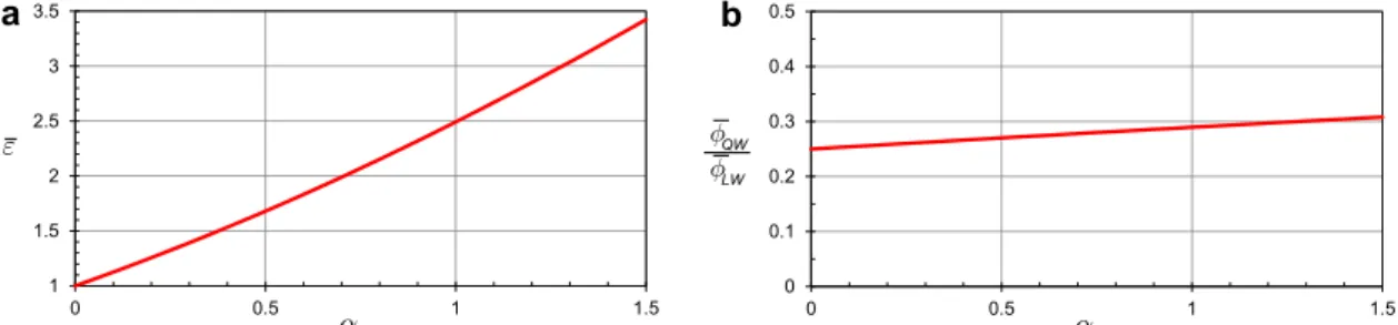
above the web (maximum) and at the free edges (minimum). Although Eq. (7) requires a matrix inversion operation, symbolic computation leads to

c c s c s II c c c I LW QW A L G A b E L G b E 2 2 2 2 2 2 2 2 4 2 2 4 , , 240 48 4 5 , 3840 64 3840 416 3                             (9)

for uncracked (I) or cracked (II) concrete, where bc is the slab total width and As/Ac is the

longitudinal reinforcement ratio. In this particular case, the solutions do not depend on x (in contrast with the previous example), but only on . The graphs in Fig. 5 plot the solutions for 01.5, making it possible to observe that approximately linear relations are obtained for the  range considered. Moreover, the mode ratios are in accordance with those reported in the previous example.

Figure 5: Variation of (a) the strain parameter and (b) the ratio of the QW/LW mode amplitudes with .

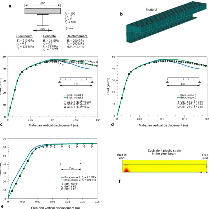
3.3 Collapse load of slender steel-concrete composite beams

Before introducing physically non-linear shear lag, two steel-concrete beams with narrow flanges are analysed, namely (i) a 6 m span simply supported beam subjected to an uniformly distributed load and (ii) a 2 m cantilever beam acted by a tip point load. The cross-section geometry and material parameters are indicated in Fig. 6(a) (mean values for C25/30 concrete are adopted). Since shear lag effects are not relevant, the GBT analyses are carried out with only 3 deformation modes (E, B and S). Preliminary analyses showed that 5 integration points are required in the web, along y, and in the concrete flange, along z (through-thickness). For comparison purposes, results obtained with brick element models (ATENA) are also presented. As in the example of Section 3.1, two refinement levels are considered, with model 2 (the most refined) involving two layers of elements in the concrete — Fig. 6(b) shows this model for the cantilever beam. To prevent transverse shear failure, a 4% reinforcement ratio is included in the concrete, along y.

refined) leading to a steeper descent. Concerning the GBT results, regardless of the number of finite elements and d value adopted, the ascending curves are in excellent agreement with the brick model ones. However, the GBT maximum load and post-peak response are significantly dependent on d, with d= 0.01 providing results that are fairly close to those obtained with the brick model 2 (the most refined). Finally, Fig. 6(d) clearly shows that the use of a mesh adjusted softening modulus effectively leads to mesh independent results and that, in this case, it suffices to employ only two elements (recall that, due to symmetry, only half of the beam is modelled).

Figure 6: Collapse load of slender steel-concrete composite beams: (a) cross-section geometry and material parameters, (b) brick element model 2, (c-d) simply supported beam load-displacement plots and (e-f) cantilever beam load-displacement

plots and equivalent plastic strain at collapse (obtained with the brick model).

Attention is now turned to the cantilever beam results, shown in Fig. 6(e). Only the results obtained with the brick model 2 are shown, but different values of the axial tensile strength fct

and fracture energy Gf are considered: (i) fct = 2.6 MPa (mean value for C25/30 concrete) and

Gf = 8.368  103 kN/m. With the GBT finite elements, the concrete is fully cracked (no

tensile strength is assumed) and the results are invariant with respect to d . For this reason, only the effect of the GBT discretization is shown in the graph. These results prompt the following remarks:

(i) Concerning the brick models, both lead to the same ultimate load, but the use of the reduced tensile strength leads to considerable lower loads along the ascending curve.

(ii) Concerning the GBT discretization, it is observed that the ascending curve requires only 4 (equal length) elements, but capturing the maximum load reasonably requires at least 8 elements. More than 16 elements lead to negligible differences.

(iii) Naturally, the ascending branch of the brick model with reduced tensile strength matches very well the GBT results. However, the maximum load is almost 7% above the GBT value corresponding to 16 elements (which, incidentally, is in accordance with a simple calculation using rectangular stress blocks). This difference can be explained with the help of Fig. 6(f), which clearly shows that the built-in support constrains plastic deformation (see [16]).

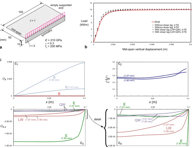
3.4 Elastoplastic steel plate with longitudinal stiffener

This example combines plasticity with shear lag and concerns the elastic-perfectly plastic simply supported stiffened steel plate shown in Fig. 7(a). Due to the double symmetry, only one quarter of the plate is analysed. The GBT analyses are carried out with the E, B and S modes, plus two additional sets of warping modes in the plate to capture shear lag effects: (i)

LW and QW or (ii) LW and 4 sinusoidal warping (SW) modes, i.e., warping modes with 1 to

4 sinusoidal half-waves along y). Integration is performed using 5 Gauss points along z and at least 6 points along y (confirmed through preliminary analyses). Due to the thin-walled nature of the plate, a refined 4-node shell (instead of brick) finite element model is employed for comparison purposes, using ADINA — see Fig. 8(a). For consistency with the GBT models, 5 Gauss points along the thickness are also considered.

The graphs (b)-(c) in Fig. 7 plot the load-displacement paths and the GBT deformation mode amplitudes. The graph (b) shows that (i) the GBT and shell results are in excellent agreement, particularly if the LW+QW modes are included in the GBT analyses, and that (ii) no more than 4 GBT finite elements are necessary to obtain accurate results. Moreover, it is concluded that the shear lag effects influence the “knee” of the load-displacement path, but not the collapse load. Although not shown in the figure, it was found that using sinusoidal warping modes yields curves that are virtually identical to those obtained with the QW mode.

The GBT deformation mode amplitude graphs c1-c4 in Fig. 7 correspond to mid-span

vertical displacements equal to 1.07 and 7.80 mm, respectively, which are associated to the first and last deformed configurations displayed in Fig. 8. These results prompt the following remarks:

(i) The c1 graph shows that the B mode has the highest participation and that the S mode

has a negligible participation. Note that, for 7.80 mm, the B mode amplitude function clearly evidences the formation of a plastic hinge at mid-span.

(ii) The c3-c4 graphs concern the warping modes. The amplitude of the E mode increases

Figure 7: Elastoplastic steel plate with longitudinal stiffener: (a) cross-section geometry and material parameters, (b) load-displacement plots and (c) GBT mode amplitude functions.

(iii) The c2 graph plots the ratio of the amplitude functions of the WQ and LW modes. It

is observed that this ratio does not vary significantly with the mid-span displacement and that the values are in quite good agreement with those previously reported for elastic shear lag (0.25 - 0.30, see Sections 3.1 and 3.2, namely Fig. 5(b)).

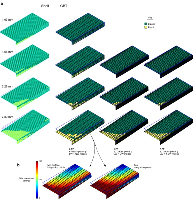
Fig. 8(a) displays the evolution of the plate deformed configuration and also the mid-surface plasticity spreading (the mid-span vertical displacement associated with each configuration is indicated in the figure). The stresses are calculated at the integration points only and no smoothing is performed.

It is observed that the GBT results are in fairly good agreement with the shell model ones and that the GBT results with LW+QW or LW+SW are very similar if 20 Gauss points are employed. The differences observed between the shell and GBT models essentially stem from the simplifications incorporated in the latter, namely the yy = 0 assumption. However, it

Figure 8: Elastoplastic steel plate with longitudinal stiffener: (a) GBT/shell deformed configurations and wall mid-surface plasticity spreading and (b) GBT deformed configurations and effective stresses at the mid-mid-surface and top

integration points.

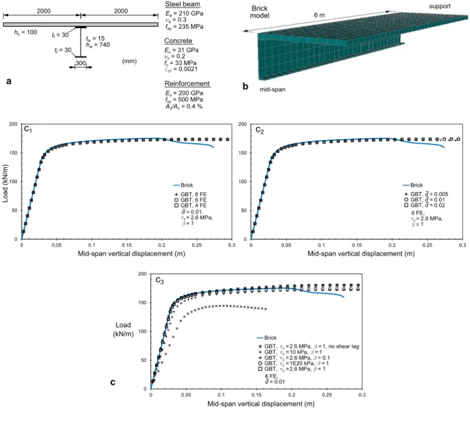
3.5 Simply supported wide flange steel-concrete beam

Figure 9: Simply supported wide flange steel-concrete beam: (a) cross-section geometry and material parameters, (b) brick model and (c) load-displacement plots.

Fig. 9(b) shows the brick finite element model analysed for comparison purposes (only 1/4 of the beam is modelled due to symmetry). As in previous cases, a 4% transverse reinforcement ratio is included in the concrete slab (besides the longitudinal reinforcement). To ensure a concrete material model as close as possible to that incorporated in the GBT element, a constant maximum shear stress is stipulated. In the ATENA program, this can be achieved by specifying that the maximum shear stress on a crack surface cannot exceed the maximum tensile stress (2.6 MPa in this case). Preliminary analyses showed the occurrence of premature localised concrete failure near the support, due to high shear forces. To prevent this failure mode and allow the development of a plastic hinge at mid-span, the concrete slab within 3 m of the support was deemed elastic (with the same Ec and c values).

The GBT analyses include the LW+QW modes and several discretisation levels and parameter values are considered. In all cases, only half of the span is modelled and 5 Gauss points are adopted along both y and z. The load-displacement graphs are displayed in Fig. 9(c), where the brick model results are also shown for comparison purposes. In particular:

(i) Graph (c1) shows the effect of the number of GBT beam finite elements, making it

although the latter predicts a load decrease after a displacement of 0.2 m. The GBT curves attain their maxima beyond that value, at 0.25-0.270 m. Nevertheless, it is remarkable that the GBT analyses provide a maximum load within 1% of the value obtained with the brick model.

(ii) Graph (c2) concerns the effect of the dparameter. No significant influence is observed

for the range analysed, although a very slight load decrease is reported for d= 0.005 and at large displacements.

(iii) Graph (c3) groups results obtained without shear lag modes (i.e., without the LW and

QW modes), as well as results for different c and  values. Concerning the shear

strength, it is concluded that using c = 10 kPa decreases the beam stiffness and

strength significantly, whereas a very high value (in this case c = 1020) leads to a

slight increase of the peak load and, naturally, to a curve virtually coincident with that obtained without shear lag modes. Concerning the  parameter, lowering it influences only the initial stages of the curve and leads to a softener response with respect to the brick model (in this particular example). The fact that the brick model agrees well with the GBT results for  = 1 may be explained by noting that, in the underlying concrete material law, although the shear stiffness decreases with cracking (as in the GBT model), the tensile strength is not zero and therefore cracking is “delayed” with respect to the GBT model — in this particular case, cracking in the brick model occurs for fairly large displacements, as discussed next.

The effect of using sinusoidal warping (SW) modes was also investigated, but the results are not shown, since no major differences were found. However, it should be mentioned that the inclusion of four SW modes (instead of a single QW mode) leads to a slight maximum load drop (almost 3%) with respect to that obtained with the QW mode. This is mostly due to the fact that the assumed GBT warping modes generate slip in the concrete/steel flange contact zone (within 150 mm of the web plane), an effect which is not allowed in the brick model (the steel/concrete interface is fully connected). If this slip is eliminated in the GBT model (which is easily achieved by subdividing the concrete slab into two 1.85 m walls and one 300 mm wall fully connected to the steel top flange), the maximum load with four SW modes drops only by 1.4%.

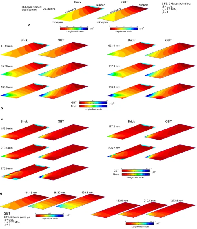
Figs. 10(a)-(c) display longitudinal strain (xx) mid-surface contour plots for one quarter of

the slab and several mid-span vertical displacement values, obtained with brick and GBT models. In the latter case, the results were obtained using the LW+QW warping modes and the discretisation/parameter values indicated in the top-right corner. It is observed that the two models yield results that are in good agreement throughout the whole displacement range (notably in the first step, still in the elastic range) and, in particular, the mid-span peak strains match quite well. However, the GBT model tends to predict a steeper transverse variation of the strains and, for the larger displacements (226.2 and 273.8 mm), does not retrieve the large localised strains obtained with the brick model.

The fact that the GBT model predicts higher strain variations in the transverse direction is a consequence of the limitation imposed on the shear stresses. In the brick model, this effect is not so pronounced, as the shear stress limitation applies to the post-cracking stresses only and significant tensile resistance is provided. To illustrate this statement, Fig. 10(d) shows results obtained assuming linear elastic shear stresses. With respect to the previous GBT results (with

c = 2.6 MPa), these surface plots are in better agreement with the brick model ones,

Figure 10: Simply supported wide flange steel-concrete beam: longitudinal strain \varepsilon_{xx} mid-surface contour plots for one quarter of the slab and a mid-span vertical displacement equal to (a) 20.05 mm, (b) 41.13 to 153.9 mm, (c)

153.9 to 273.8 mm and (d) 41.13 to 273.8 (GBT results without shear stress limitation).

Figure 11: Simply supported wide flange steel-concrete beam: evolution of cracking as the mid-span vertical displacement increases (brick model).

4 CONCLUDING REMARKS

In this paper, a computationally efficient physically non-linear GBT-based finite element for steel and steel-concrete beams was proposed and validated. The element is able to capture the materially non-linear behaviour of wide-flange steel and steel-concrete composite beams up to collapse, including reinforced concrete non-linear material behaviour, shear lag effects and steel beam plasticity. A set of numerical examples were presented, in order to demonstrate that the finite element is capable of capturing all relevant phenomena with a very small computational cost. Furthermore, analytical solutions for elastic shear lag were derived and the unique modal decomposition features of GBT were employed to extract information concerning the shear lag effect in both the linear and non-linear stages, up to collapse.

It should be mentioned once again that the efficiency of the proposed element stems from a combination of the GBT intrinsic versatility to model the behaviour of thin-walled members and the introduction of specific assumptions concerning the stresses and strains. These assumptions make it possible to reduce the number of cross-section deformation modes (and, hence, reduce DOFs) and also employ simple constitutive laws for both steel and concrete, without sacrificing accuracy. Finally, a few words concerning the computation times. With an Intel Core i7 CPU @ 2.10 GHz processor, the GBT analyses typically run under 1 or 2 minutes, whereas the ATENA analyses can take more than 12 hours if extensive cracking occurs in the concrete slab.

REFERENCES

[1] Schardt R., “Eine erweiterung der technischen biegetheorie zur berechnung prismatischer faltwerke”,Stahlbau, 35, 161-71, 1966 (German).

[2] Schardt R. Verallgemeinerte Technische Biegetheorie, Springer-Verlag, Berlin, 1989 (German).

Stability and Ductility of Steel Structures, E. Batista, P. Vellasco, L. Lima (eds.), Rio de Janeiro, Brazil, 33-58, 2010.

[4] Nedelcu M., “GBT formulation to analyse the behaviour of thin-walled members with variable cross-section”,Thin-Walled Structures, 48(8), 629-38, 2010.

[5] Camotim D., Basaglia C., Silva N. and Silvestre N., “Numerical analysis of thin-walled structures using generalised beam theory (GBT): recent and future developments”, Computational Technology Reviews, vol.1, B. Topping, J. Adam, F. Pallarés, R. Bru, M. Romero (eds.), Saxe-Coburg, Stirlingshire, 315-54, 2010.

[6] Camotim D. and Basaglia C., “Buckling analysis of thin-walled steel structures using generalized beam theory (GBT): state-of-the-art report”, Steel Construction, 6(2), 117-31, 2013.

[7] Gonçalves R. and Camotim D., “Steel-concrete composite bridge analysis using generalised beam theory”,Steel & Composite Structures, 10(3), 223-43, 2010.

[8] Bathe K.J., ADINA system, ADINA R&D Inc., 2012.

[9] Cervenka V., Jendele L. and Cervenka J., “ATENA 3D program documentation”, Cervenka Consulting, 2013.

[10] Gonçalves R. and Camotim D., “Generalised beam theory-based finite elements for elastoplastic thin-walled metal members”, Thin-Walled Structures, 49(10), 1237-45, 2011.

[11] Gonçalves R. and Camotim D., “Geometrically non-linear generalised beam theory for elastoplastic thin-walled metal members”, Thin-Walled Structures, 51, 121-9, 2012.

[12] Gonçalves R., Ritto-Corrêa M. and Camotim D., “A new approach to the calculation of cross-section deformation modes in the framework of Generalized Beam Theory”, Computational Mechanics, 46(5), 759-81, 2010.

[13] Gonçalves R., Bebiano R. and Camotim D., “On the shear deformation modes in the framework of Generalized Beam Theory”,Thin-Walled Structures, 84, 325-34, 2014.

[14] EN1992-1-1:2004, Eurocode 2: design of concrete structures - Part 1-1: general rules and rules for buildings, CEN, Brussels, Belgium, 2004.

[15] MATLAB, version 7.10.0 (R2010a), The MathWorks Inc., Massachusetts, 2010.

[16] Gonçalves R., Coelho T. and Camotim D., “On the plastic moment of I-sections subjected to