1
A Work Project, presented as part of the requirements for the Award of a
Master’s Degree in Economics from the NOVA –
School of Business
and Economics
Labor mobility in Belgium:
A Panel VAR approach
Robin Hublet
Student no. 29379
A project carried on the Master’s in Economics Program under the supervision of: Professor Francesco Franco
2
ABSTRACT
This research investigates labor market dynamics in Belgium and the specific role played by labor mobility in the adjustment process following a labor demand shock. It first analyzes the time series characteristics of the Belgian labor market based on a panel of 11 provinces from 2003 to 2015. This analysis allows the building and estimation of a PVAR model to obtain the response of employment, employment rate, and labor force participation rate to a shock in labor demand. The results suggest a minor role played by migration in the first years of the adjustment process, highlighting the difficulties for the EU to be considered an OCA.
Keywords: European Union, OCA, Labor Mobility, PVAR Estimation.
1. Introduction
Since the outburst of the economic and financial crises, the importance of macroeconomic adjustment mechanisms as a tool to counteract crises has reemerged in the economic debate. When monetary unions such as the United States (US) or the European Union (EU)1 face economic downturns, adjustments are needed to resolve labor market issues, often characterized by a high unemployment rate.
Unemployment rates in Europe have recently been of particular interest due to their increased divergence among European countries and regions. In 2016, the unemployment rate was as high as 22% in Greece and 19% in Spain while it only stood at 4% in Germany and 8% in Belgium. Those high differences among European countries are not only present at the country level but appear even more pronounced at a regional level. In Germany, for example, the highest regional unemployment rate for the same year was almost four times that of the best performing region. In Greece, the highest value went up to 31% while the region’s lowest rate was only half of that value at 16% (Eurostat, 2017).
3
The apparent difficulty of European countries and regions in eliminating quickly those high disparities has given more attention to the importance of labor mobility as a means of adjustment. A central question then arises: is there a lack of labor mobility in the EU that could explain the high persistency of unemployment in economically depressed regions? The answer to this question is of crucial importance for policy makers aiming at better facing next economic crises in the EU.
This paper tackles this question, contributing to the growing labor mobility debate in Europe by modelling a panel vector autoregression (PVAR) model based on the approach used in Blanchard and Katz (1992). This approach investigates how labor market variables such as employment, unemployment, and labor force participation respond to asymmetric shocks in labor demand, and whether labor mobility plays an essential role in helping with this adjustment. Using a panel of 11 provinces in Belgium from 2003 to 2015, this paper finds that labor force participation plays an essential role in the adjustment process in the first years following the shock while migration plays a smaller role. The results confirm the current labor market difficulties encountered by EU countries in adjusting quickly after a demand shock.
4
2. Literature review
The usefulness of labor mobility as adjustment process against asymmetric shocks in a monetary union is a subject undergoing intense study in the academic debate today. The inability of the EU to resolve quickly and effectively the two consecutive crises of 2008 and 2012 has led to the reemergence of the theory of Optimal Currency Areas (OCA). This theory introduced by Robert Mundell in 1961 has developed considerably over the years leading to major empirical works. This literature review looks at the most important theoretical and empirical evolutions of the OCA literature over the last decades and illustrates how this paper complements it.
2.1. Theoretical works
An OCA is defined by different criteria including labor mobility, capital mobility, wage and price flexibility, openness of the economy, similarity of business cycles, fiscal integration and political integration. Those criteria were built on the basis of three pioneering papers by Mundell (1961), McKinnon (1963), and Kenen (1969). These three authors defined an OCA as a region where it would be optimal to have a single currency. First, Mundell (1961) set a classical view on OCA in his paper “A theory of Optimal Currency Areas”. When investigating the
5
Mundell (1961) suggested various preconditions for the formation of such an area, emphasizing primarily the need for high internal factor mobility. Labor mobility is crucial when certain regions face economic downturns as it allows unemployed people to move to economically stable regions. This movement of workers helps reduce the unemployment burden of depressed regions while putting pressure on inflation in booming areas, this enables economically-hit regions to recover their competitiveness more quickly. This theory, however, has recently been challenged by Farhi and Werning (2014) who state that depressed regions facing less labor supply might be affected by a worsened purchasing power. The authors highlight that the effects on the population staying in the depressed region will be highly dependent on the way the region relies on internal or external demand.2 If it relies on external demand, the region might find itself in a better position after the out-migration of its labor supply, while if it relies on internal demand, labor out-migration might have a less pronounced impact on the depressed region. Indeed, when workers migrate out of the region, this reduces the labor supply, while it also reduces the demand for non-traded goods, this in turn lowering the demand for labor. Those two effects cancel each other, leaving the region in the same position as before. This argument is in line with the second building block of the OCA classical theory, initially stressed out by McKinnon (1963). McKinnon (1963) argues that regions or countries should form a currency union if they are strong trading partners. Finally, Kenen (1969) emphasizes the necessity of transfers between regions. The involvement of transfers from regions doing well to regions experiencing more difficulties is often seen as the other crucial missing criterion in the EU today. Those transfers are central for helping regions that are hit by a shock recover more easily and quickly. In line with this argument, Farhi and Werning (2017) argue for fiscal transfers in
2 Internal demand comes from goods produced in the region, while external demand comes from goods produced in
6
currency unions as an optimal international risk-sharing arrangement, providing macroeconomic stabilization effects. They emphasize three key determinants for the stabilization performance: the asymmetry of the shocks, the persistence of these shocks, and the openness of the member countries or regions. Fiscal transfers having more significance when shocks are asymmetric, the persistence of these shocks is large, and the economy is more closed.
The amount of literature on OCA during the seventies and eighties declined. Nevertheless, after the Maastricht Treaty in 1992 set the path for a monetary union in the EU, the interest rose among researchers to assess how the future European Monetary Union (EMU) would look like. De Grauwe (1993) looked into the costs and benefits from such a union. He underlined the great disparity already present between economies such as Germany and Italy or Spain, stating that the benefits might be greater for countries like Italy and Spain as the EMU would provide them with a more stable and low inflation environment. On the contrary, the costs for a country like Germany to join the monetary union would be great as it would undermine its reputation and leave it with less power on monetary policies. This contrast between countries highlights the conflicts in political and economic objectives involved in the Maastricht Treaty.
7
Two decades later, the economic and financial crises of 2008 gave a new impulse to the study of OCA with the work of Krugman (2012) as main contributor to the subject. Analyzing the flaws of the EU to respond quickly to the crisis, the author claims that EU leaders failed to anticipate the inevitable. Further building on the literature of Mundell (1961) and Kenen (1969), he addresses their two main contributions, namely labor mobility and fiscal integration, by showing how US states have dealt with asymmetric shocks in the past. The author takes the example of Florida to illustrate how efficient the US labor market responds to asymmetric shocks by having automatic compensating transfers that enable to relieve the burden of a crisis on states experiencing economic downturns. The crucial point of fiscal transfers in a Federal country like the US is that the federal government does not face a borrowing problem if one state experiences difficulties, and has very low borrowing costs. This would not be the case if Florida was a sovereign country. Furthermore, although Krugman (2012) does not see labor mobility to be as important as fiscal transfers to combat asymmetric shocks, he argues that labor mobility should have played a larger role in the economic recovery of the euro area, especially for countries such as Spain. He illustrates his argument with the case of Massachusetts, a US state that experienced a major economic shock in the end of the 1980’s. The author shows through an analysis of the
8
the crisis in 2008 with high emigration rates experienced in Spain, Portugal, and Greece as pointed out by the “2016 Annual Report on intra-EU Labor Mobility” (Fries-Tersch, Tugran and Bradley, 2016). Furthermore, many suggestions to promote labor mobility in the EU have emerged in the literature. An example comes from De Wispelaere and Pacolet (2015) who bring forward the idea of posting workers, defined as an activity of an employee for his/her employer which is temporarily exercised outside the Member State where the employer is established.
2.2.Empirical works
Turning to the recent empirical literature on labor mobility and its importance as adjustment mechanism, the most influential studies focus on the differences between the US and the EU. The US provide a great case of study as it is a Federal country based on a single currency over a very large number of states while the EU is interesting as its relative recent history provides great opportunities for improvement. However, the lack of reliable data has made it difficult for economists to estimate labor mobility. Two ways of measuring labor mobility have emerged in the literature, a direct and an indirect way. The former method tries to measure labor mobility through surveys, often conducted over a restricted number of people. The latter method tries to measure labor mobility through the estimation of the joint movement of various labor market variables, it is also the method used in this paper.
9
Europe, this is the case of the EU-Labor Force Survey (EU-LFS) which is a large household survey providing quarterly results on labor force participation of people aged 15 and above, that covers the years 1983 onwards. The “2016 Annual Report on intra-EU Labor Mobility” uses this survey to look at the current trends in labor mobility in the EU.
The interest in the literature has slowly shifted to other measurement methods not relying exclusively on surveys. A first influential paper by Eichengreen (1991) came in the early nineties and tried to look at the speed of adjustment of the labor market and labor mobility in the US compared to the EU. At that time, the author pointed out the EU as less of an OCA compared to North-America, namely the US and Canada. His results suggest a 20 percent faster adjustment rate in the US.
10
demand. The authors find evidence that migration is an important part of the adjustment process in the US. This paper bases itself on the model proposed by Blanchard and Katz (1992).
Many papers have used the same empirical methodology as Blanchard and Katz (1992). This is the case of Decressin and Fatas (1995), and Obstfeld and Peri (1998) who analyze regional labor dynamics in Europe and compare them to the results obtained for the US. They both find that the adjustment to labor demand shocks transpires more through labor mobility in the US than in the EU while in the EU a big part of the adjustment in the first years after an adverse shock is done by a decreased participation rate. Decressin and Fatas (1995) further verify whether this smaller role played by migration in the EU might be due to people’s difficulties in
moving across countries. After checking for the interregional migration for the United Kingdom (UK), Germany, and Italy, they find little interregional migration even within those countries.
Furthermore, other papers have used this method to investigate country specific regional evolutions such as Mäki-Arvela (2003), and Alecke, Mitze, and Untiedt (2010), who analyze regional evolutions in Finland and Germany respectively. Finally, two influential papers estimate the same model for Spain: Jimeno and Bentolila (1998), and Sala and Trivin (2014). Both papers find that migration plays a smaller role in the adjustment process in Spain compared to the US but the latter finds an increased role played by the labor force participation in the adjustment process. It seems thus that all papers find a lower role played by labor mobility in the adjustment process in the EU compared to the US, however, Beyer and Smets (2015) find a convergence tendency, with labor mobility increasing over time in the EU and decreasing in the US.
11
role is still debated in the literature today. The empirical literature focuses on this last point by trying to estimate the role played by labor mobility when a currency union faces an asymmetric shock. It is also what this paper tries to accomplish.
3. Regional evolutions and time series analysis
This research uses a panel of 11 provinces of Belgium (Brussels, Antwerp, West-Flanders, East-West-Flanders, Limburg, Flanders-Brabant, Walloon-Brabant, Hainaut, Liège, Namur, and Luxembourg) over 12 years of yearly data (from 2003 to 2015), to estimate the role that labor mobility plays in Belgium after an adverse shock in labor demand. 3
It is first important to stress out that the choice of Belgium as country of interest was not taken arbitrarily but rather because Belgium characterizes on a small scale the cultural and linguistic diversity of Europe. Indeed, one issue found in the study of labor mobility in the EU is the lack of explanation for the lower mobility in the EU compared to the US. Eichengreen (2014) points to specific problems in the EU including: differences in languages, limited access to local healthcare and benefits, and uncertainties regarding the transfer of pension rights. Indeed, it the choice of moving is interlinked with many different economic, demographic, and socio-cultural characteristics (Bonin et al, 2008). The language and socio-cultural barriers encountered in the EU appear to be determinant when individuals choose to move, explaining in some part why the labor mobility is so limited in the EU, as expressed by Zimmerman (2009). Belgium provides in this sense, an optimal place of study for two main reasons. First, it is a Federal country meaning that each region has a high degree of self-governance under the authority of the Federal government which is in line with the governing independence of EU countries. Secondly, Belgium is characterized by a high degree of cultural and linguistic differences. Indeed, Belgium
12
is divided in three culturally different areas; a Dutch-speaking part in the North, a French-speaking part in the south, and a bilingual (French/Dutch) part in the center.4 By analyzing a country culturally divided, this paper addresses the issue of diversity in the EU.
The rest of this section describes the labor market dynamics in Belgium. Furthermore, the detailed analysis of the time series specifications of employment, unemployment, and wages is performed based on the simple model proposed by Blanchard and Katz (1992).5 This is important for the estimation of the PVAR model in the next section.
3.1. Relative Employment: trends and characteristics
Over the past decade, Belgian provinces have shown sustained differences in their employment growth rates. Figure 1 illustrates this by plotting the average employment growth from 2003-2009 against average employment growth from 2010-2015, where annual employment growth is measured by the average annual change in log employment over the specified period. The positive correlation between both periods shows that provinces have experienced persistent differences in employment growth rates, however, the differences are relatively small ranging from 0.4% to 2% for the period 2003-2009, while ranging from 0.2% to 1.2% for the period 2010-2015. This low variation in growth rates contrasts with the results obtained by Blanchard and Katz (1992) for the US, and confirms that variation in growth rates are usually smaller in EU countries. Furthermore, it seems that Walloon-Brabant has consistently grown faster than the average and that Brussels on the contrary has been lagging behind. Lastly, it can be remarked that for both periods, provinces part of Flanders tend to grow faster than provinces in Wallonia.
4 North (Flanders) includes: Antwerp, West-Flanders, East-Flanders, Limburg, and Flanders-Brabant. South
(Wallonia) includes: Walloon-Brabant, Hainaut, Liège, Luxembourg, Namur, and Luxembourg. Center includes: Brussels.
13
Figure 1. Persistence of Employment Growth rates across Belgian Provinces, 2003-2015
Source: Calculations using Employment NUTS2 regions. See section A.1. of the appendix for more information on the data. BXL Brussels, ProvANTW Antwerp, ProvLim Limburg, ProvOVL East-Flanders, ProvWVL West-Flanders, ProvVLBRB Flanders-Brabant, ProvWALBRB Walloon-Brabant, ProvNAM Namur, ProvHN Hainaut, ProvLG Liège, ProvLX Luxembourg.
Furthermore, figure 2 takes a look at the regional trends and fluctuations of relative employment in Belgium by showing the evolution of employment of the different provinces relative to the Belgian aggregate employment. Figure 2(a) presents the five provinces of Flanders plus Brussels. It appears that the Flemish-Brabant and Limburg have been the most hit by the economic crisis in 2008. While the former has shown constant upward trend, the latter has experienced a downward movement over the years. Figure 2(b) portrays the five provinces of Wallonia plus Brussels. The range of volatility in the time series looks similar to Flanders, however, Walloon-Brabant strikes out as it exhibits a very upward trend over the years.
It appears that in both figures 1 and 2, Walloon-Brabant shows an increasing employment growth. The results obtained translate the high demographic growth in the province for the past twenty years (FESBW, 2015). Indeed, Walloon-Brabant has the fastest demographic growth of Belgium, highly dependent on migration flows from other Belgian provinces. Brussels, on the other hand, experiences the lowest employment growth of the country. This also translates the demographic outflows that Brussels has experienced for the past two decades.
BXL ProvANTW
ProvHN ProvLG
ProvLXProvLim
ProvNAM ProvOVL
ProvVLBRB
ProvWALBRB
ProvWVL
.2
.4
.6
.8
1
1
.2
.5 1 1.5 2
14
Figure 2. Cumulative Employment Growth, Province relative to National Average, 2003-2015
Source:Calculations using Employment NUTS2 regions. See section A.1. of the appendix for more information on the data.
The two figures presented above give a broad and first look at the employment growth in Belgium. In order to have a better understanding of the stochastic behavior of relative employment, this paper analyzes a formal characterization of the time series for relative employment. Figure 1 and 2 appear to present non-stationarity in the time-series, and some provinces seem to exhibit a trend. In order to test for stationarity, this paper looks at the presence of a unit-root by running for each province
∆𝑛𝑖𝑡 = 𝛼1𝑖+ 𝛼2𝑖(𝐿)∆𝑛𝑖,𝑡−1+ 𝜀𝑖𝑡 (1) Where 𝑛𝑖𝑡 is the logarithm of employment in province i at time t minus the logarithm of employment in Belgium at time t, 𝛼1𝑖 is a constant term, and 𝜀𝑖𝑡 is a disturbance term.
The augmented Dickey-Fuller (ADF) test was run with a trend component, however, it did not appear significant when running the test. Therefore, a trend component was not included when running the test. Running the Partial Autocorrelation gives an indication on the number of lags to choose, indicating that one lag is sufficient. The results obtained show that all coefficients are negative apart from two provinces. The hypothesis of a unit root is not significant at a five percent level for all the provinces apart from Brussels and East-Flanders. This result appears to indicate non-stationarity in the data. Therefore, in the remaining of the paper the first-difference
-4
-2
0
2
4
2003 2015
Year
BXL ProvVLBRB ProvANTW ProvLim ProvOVL ProvWVL
(a)
-5
0
5
10
15
2003 2015
Year
BXL ProvWALBRB ProvNAM ProvHN ProvLG ProvLX
15
of relative employment is taken. This transformation gives stationary data for all provinces. Next, a univariate process for relative employment is built by running from 2003 to 2015:
∆𝑛𝑖𝑡 = 𝛼1𝑖+ 𝛼2𝑖(𝐿)∆𝑛𝑖,𝑡−1+ 𝜀𝑖𝑡 (2) Allowing for two lags in 𝛼2𝑖(𝐿), the estimated coefficients are calculated from which an associated impulse response is derived. This estimation gives the response of the level of relative employment to an innovation in 𝜀. Table 1 gives the results that were obtained by pooling all provinces together and allowing for province fixed effects – that is, different constant terms for each province. Pooling all provinces together enables to take advantage of the cross section and time series dimensions of the data. Furthermore, since the time span of the data is short, pooling the data allows for more degrees of freedom.
Table 1. Univariate Models of Relative Employment, Unemployment, and Wages
Result Relative Employment Relative Unemployment Relative Wage Coefficient on lagged
dependent variable
One Lag -0.06 0.196 0.462
(-0.103) (-0.069) (-0.09)
Two Lags 0.034 0.029 0.272
(-0.096) (-0.067) (-0.856)
Implied Impulse Responses
Year 1 1 1 1
Year 2 0.94 0.2 0.46
Year 3 0.92 0.07 0.49
Year 4 0.89 0.02 0.35
Year 5 0.87 0.01 0.29
Year 10 0.75 0 0.08
Year 20 0.58 0 0.01
Source: Estimates of univariate equations using data described in the appendix. Standard errors of the coefficients are in parentheses. All corresponding graphs of the impulse responses can be found in section A.2. of the appendix.
16
To sum up, relative employment in Belgium is characterized by different rates between provinces, where shocks have permanent effects, or at least appear to come back to trend very slowly.
3.2. Relative Unemployment: trends and characteristics
Taking a look at relative unemployment rates, it can be noted that there exists a high persistency over the years in Belgium. Figure 3 portrays the persistence of relative unemployment per province, taking the mean of relative unemployment rate in 1999 against the mean of relative unemployment rate in 2015.
Figure 3. Persistence of Relative Unemployment Rates across Belgian Provinces, 1999-2015
Source:Calculations using Unemployment NUTS2 regions. See section A.1. of the appendix for more information on the data.
Results show strong persistency over the years with a slope of 0.93 and R² of 0.88. Those results contrast with the finding of Blanchard and Katz (1992) for the US, however, it resembles the findings of Mäki-Arvela (2003) for Finland. This higher persistency in Belgium is also in line with the work of Bertola & Ichinov (1995) who find evidence of stronger persistency in unemployment rates in Europe by looking at the UK, France, and Italy and comparing the results obtained to the ones of Blanchard and Katz (1992) for the US. Explanations for higher persistency in unemployment rates often touch upon the labor market rigidities encountered in
BXL
ProvANTW
ProvHN ProvLG
ProvLX
ProvLim
ProvNAM
ProvOVL ProvVLBRB
ProvWALBRB
ProvWVL
5
10
15
20
5 10 15
17
the EU, impeding quick adjustments to shocks through wage cuts. Furthermore, it can be noticed that Brussels is the worst performer in both years, while provinces from Flanders seem to show better results than provinces from Wallonia.
Turning to the formal characterization of the relative unemployment rate, this paper examines the same equation as (1), only changing 𝑛𝑖𝑡 by 𝑢𝑖𝑡; the unemployment rate in province i at time t minus the Belgian unemployment rate at time t. The stochastic behavior of relative unemployment rate is analyzed by running the ADF test for each province. The null hypothesis of a unit root is not significant at a five percent level for all provinces apart from one. However, based on theoretical grounds, the prior that relative unemployment rates are stationary is considered by using the level rather than the first difference of the relative unemployment rate in the remaining of this paper. In addition, the estimation of the univariate process for relative unemployment is estimated with its corresponding impulse responses. This estimation is done by pooling the data of all provinces, allowing for province fixed effects, and two lags. As shown in table 1, relative unemployment seems to get back to its trend very quickly after a shock.
Summing up, relative unemployment seems to be persistent over the years with clear differences observed between Flanders and Wallonia. Furthermore, the impact of a shock appears to be quickly overcome within three years.
3.3. Convergence of Relative Wages
18
Figure 4. Convergence of Relative Wages in Belgium, 2003-2015
Source:Calculations using Compensation NUTS2 regions. See section A.1. of the appendix for more information on the data.
As shown by the negative slope of the regression line, Belgian provinces performing the worst in the starting year are the ones performing the best during the entire period. This indicates that relative wages have been converging over the period analyzed in Belgium.
Furthermore, the stochastic behavior of relative wages is also examined by running the same equation as (1) but changing 𝑛𝑖𝑡 by 𝑤𝑖𝑡; the logarithm of wage in province i at time t minus the aggregated value of Belgium. Running the ADF test, the hypothesis of a unit root is not significant at five percent level for all states but one, however, based on theory the level of relative wages is used rather than first differences in the remaining of this paper. Lastly, the specification of the autoregressive process, allowing for two lags and pooling the provinces together, offers the possibility to look at the impulse responses of a shock in relative wages. Table 1 shows that relative wages appear to have the same tendency as relative unemployment rates in coming back to trend in a few years, however, they seem to take more time; approximately ten years.
BXL ProvANTW
ProvHN ProvLG ProvLX
ProvLim ProvNAM
ProvOVL
ProvVLBRB ProvWALBRB
ProvWVL
1
.8
1
.9
2
2
.1
2
.2
2
.3
10.2 10.3 10.4 10.5 10.6 10.7
19
4. PVAR model estimation: simulated dynamic responses
The results obtained for the relative unemployment rate show that deviations of relative unemployment rates from their means are not persistent in Belgium. This suggests that relative employment shocks might not be absorbed by changes in relative unemployment. Blanchard and Katz (1992) find for the US that the rapid return to long-term means of relative unemployment and relative participation rates is mainly explained by an out-migration of workers when a region is hit by a labor demand shock. Moreover, Decressin and Fatas (1995) find that, in Europe, most of the adjustment after a shock happens through a decline in the labor force participation.
This section investigates how shocks to regional labor demand are absorbed across Belgian provinces by running a PVAR model estimating the joint behavior of relative employment, relative employment rate, and relative participation rate and deriving the corresponding impulse response functions from the estimates. The responses provide information on the role played by migration in the adjustment process. Indeed to the extent that labor demand shocks are not reflected in employment rate or participation rate changes, they must be absorbed by inter-provincial migration. The results obtained are further compared to some of the main findings in the empirical literature today for the US and the EU.
The PVAR model estimated in this paper takes the following form:6
∆𝑒𝑖𝑡 = 𝛼𝑖10+ 𝛼𝑖11(𝐿)∆𝑒𝑖,𝑡−1+ 𝛼𝑖12(𝐿)𝑙𝑢𝑖,𝑡−1+ 𝛼𝑖13(𝐿)𝑙𝑝𝑖,𝑡−1+ 𝜀𝑖𝑒𝑡 (3) 𝑙𝑒𝑖𝑡 = 𝛼𝑖20+ 𝛼𝑖21(𝐿)∆𝑒𝑖𝑡+ 𝛼𝑖22(𝐿)𝑙𝑢𝑖,𝑡−1+ 𝛼𝑖23(𝐿)𝑙𝑝𝑖,𝑡−1+ 𝜀𝑖𝑢𝑡 (4) 𝑙𝑝𝑖𝑡 = 𝛼𝑖30+ 𝛼𝑖31(𝐿)∆𝑒𝑖𝑡+ 𝛼𝑖32(𝐿)𝑙𝑢𝑖,𝑡−1+ 𝛼𝑖33(𝐿)𝑙𝑝𝑖,𝑡−1+ 𝜀𝑖𝑝𝑡 (5) Where ∆𝑒𝑖𝑡 is the difference of the logarithm of employment in province i minus the first-difference of the logarithm of employment for Belgium, 𝑙𝑒𝑖𝑡 is equal to the logarithm of the ratio of employment to the labor force in province i minus its counterpart for Belgium, and 𝑙𝑝𝑖𝑡 is
20
equal to the logarithm of the ratio of labor force to the working age population of province i minus its aggregated value for Belgium.Furthermore, 𝛼𝑖 and 𝜀𝑖 are constants and idiosyncratic error terms, respectively. This dynamic PVAR model assesses how the different variables adjust in response to a shock in labor demand, identified in this model as 𝜀𝑖𝑒. This model identification assumes that unexpected movements in employment within the year primarily reflect movements in labor demand rather than labor supply. 7 The model allows for two lags for each variable. Like Blanchard and Katz (1992), all provinces are pooled together, allowing for province-fixed effects, thus estimating the dynamics of the average province. Considering the small range of data of the estimation, pooling the data increases the number of data points and degrees of freedom, thereby giving more reliable results.
The lag structure of the model allows current changes in ∆𝑒𝑖𝑡 to affect contemporaneously the values of relative employment rate and relative participation rate, but not the other way around. After the PVAR estimation is completed, the computation of the impulse responses is performed, which describe the dynamic effects of a shock in labor demand on relative employment, relative employment rate, and relative participation rate. The responses of a one standard deviation shock in relative employment growth are plotted in figure 5.8 All
responses obtained present the expected shape and signs. The interest, however, resides in the
magnitude of the responses to assess the importance of relative employment rates, relative
participation rates, and migration in the adjustment process following a labor demand shock.
7
Further explanation and proof can be found in section A.5. of the appendix.
8 All PVAR estimations and resulting impulse responses are estimated using the package provided by Ryan Decker,
which is an update of the original package developed by Inessa Love and used in Love and Zicchino (2006). The
21
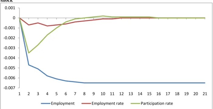
Figure 5. Responses of Employment, Employment rate, and Participation rate to an Employment shock
Source: Calculations based on System OLS. The shock is -1 standard deviation to relative employment.
Confidence intervals are provided in section A.8. of the appendix.9
The results of figure 5 show that, in Belgium, an adverse shock of one standard deviation
decreases relative employment by 0.47 percentage points, relative employment rate by 0.07
percentage points, and relative participation rate by 0.35 percentage points. It appears that in
Belgium, almost all adjustment after the shock is taken by a strong decrease in labor force
participation in the first four years. Indeed, the relative participation rate decline accounts for as
much as 75 percent of the adjustment in the first year while the relative employment rate only
takes a small role accounting for 15 percent of the adjustment in the first year. The implied
out-migration of workers in the first year following the shock is thus a small 10 percent of the
adjustment. Over the course of the first four years, participation’s role as adjustment slowly
9While Blanchard and Katz (1992) compute the response of relative unemployment rate after the estimation of the
model, this paper shows the response of relative employment rate. The two are equivalent, however, the estimation using relative employment rate gives more reliable confidence intervals. The formal proof based on Decressin and Fatas (1995) can be found in section A.7. of the appendix.
-0.007 -0.006 -0.005 -0.004 -0.003 -0.002 -0.001 0 0.001
22
decreases to let out-migration be the main source of adjustment after four years. It takes about
nine years for the effect of the demand shock to be totally accounted for by out-migration.
Those results reflect the recent empirical findings in the literature, namely that labor force
participation in the EU plays a major role when labor demand is hit by an adverse shock. Indeed,
many papers focusing on the EU and individual EU countries have found the same pattern. Table
2 summarizes the main empirical findings present in the literature by showing the
decompositions of the impulse responses. The values presented reflect the shares played by
relative employment rate, relative participation rate, and migration in the adjustment process.
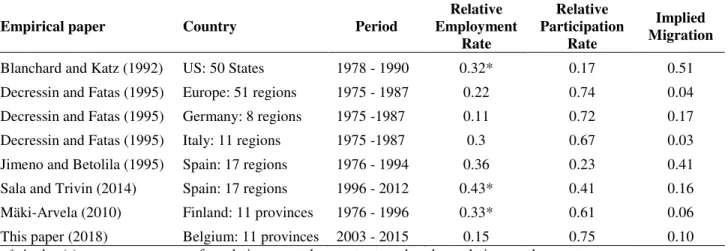
Table 2. Impulse Response decomposition of a one standard deviation Relative Employment shock
Empirical paper Country Period
Relative Employment
Rate
Relative Participation
Rate
Implied Migration
Blanchard and Katz (1992) US: 50 States 1978 - 1990 0.32* 0.17 0.51 Decressin and Fatas (1995) Europe: 51 regions 1975 - 1987 0.22 0.74 0.04 Decressin and Fatas (1995) Germany: 8 regions 1975 -1987 0.11 0.72 0.17 Decressin and Fatas (1995) Italy: 11 regions 1975 -1987 0.3 0.67 0.03 Jimeno and Betolila (1995) Spain: 17 regions 1976 - 1994 0.36 0.23 0.41 Sala and Trivin (2014) Spain: 17 regions 1996 - 2012 0.43* 0.41 0.16 Mäki-Arvela (2010) Finland: 11 provinces 1976 - 1996 0.33* 0.61 0.06 This paper (2018) Belgium: 11 provinces 2003 - 2015 0.15 0.75 0.10
* Author(s) compute responses for relative unemployment rate rather than relative employment rate.
When comparing results for the EU and the US, the main differences reside in the
different roles played by labor participation and migration. Moreover, in the EU, the role played
by migration is not substantial in the first year after the shock while it plays a significant role in
the US. Indeed, the results obtained by Blanchard and Katz (1992) show that as much as 51
percent of the adjustment is borne by out-migration of workers in the first year. This high
percentage is only approached by Jimeno and Betolila (1995) who find that migration accounts
for 41 percent of the adjustment in the first year. In 2014, however, Sala and Trivin challenged
23
adjustments via changes in participation rates are much more relevant today than in the past. At
the same time, they get much lower results for the role of migration. The results of this paper
closely ressemble the ones obtained by Decressin and Fatas (1995) for Germany, with a minor
role played by relative employment rate in the adjustment process, and a very prominent role
played by relative participation rate. Furthermore, migration in Belgium appears to have a much
smaller role in the short-run adjustment process when compared to the US. The small adjustment
role played by migration in Belgium is thus not unexpected when comparing it to other European
countries such as Finland, Germany, Italy, or Spain. As table 2 illustrates, the magnitude of the
adjustment via labor mobility in the EU seems not only to be small across EU countries but also
within countries, as this paper confirms.
To go further, the importance of relative wages in the adjustment process might have
implications for the labor market adjustment. This paper finds a small role played by relative
wages after a shock in relative employment.10
6. Discussion and limitations of the results
The results obtained for Belgium indicate that labor mobility within the country does not have a significant impact in the adjustment process after a shock in demand. Those results are in accordance with many empirical papers for other EU countries. The responses of the participation rate and employment rate to the demand shock might find some explanations in the way the labor market is constructed in Belgium.
Concerning the labor force participation, the fact that workers massively withdraw from the labor market after a demand shock has been argued by Decressin and Fatas (1995) as a general tendency in the EU. The authors explain that this trend might be due to the fact that employers in the EU considerably rely on early retirements to adjust the size of the workforce in
24
difficult periods. This argument is partially confirmed by the increased early retirements observed in the economy in Belgium (SPFE, 2013). Furthermore, Decressin and Fatas (1995) also highlight the fact that women in the labor force are usually more likely to leave the labor force when a shock to the economy happens as they are on average employed in low skill positions implying lower compensation costs. Those arguments might thus explain some of the high role played by participation rates in the aftermath of a demand shock.
Looking at the employment rate, its limited role as adjustment mechanism might be explained by the role played by part-time jobs during crises in Belgium. As expressed by the recent study conducted by the Service Public Fédéral Économie (SPFE), during the recent crisis, the number of full-time jobs decreased, but this decline was partially compensated by an increase in part time jobs. This increase relieved the economy from massive layoffs.
25
methods are very recent in the empirical literature and the results derived from them have thus to be taken with caution.
7. Conclusion
This paper investigated and estimated the response of the Belgian labor market to a shock
in labor demand. This paper began by analyzing the main characteristics of the Belgian labor
market by looking at the behavior of employment growth, unemployment, and wages. This
analysis pointed out: different employment growth rates, high disparity and persistency in
unemployment rates, and converging wages between Belgian provinces. After estimating the
time series properties of the labor market and checking for stationarity, this paper investigated
the effects of a labor demand shock on provincial employment level, employment rate, and labor
force participation rate. The results show that a labor demand shock permanently decreases the
employment share of a province, showing that in the long-run workers migrate out of the
province to go to booming labor market provinces. Nonetheless, the role played by migration in
the first years after the shock is very restricted. It appears that the strongest role played in the
adjustment is the decrease of the labor force participation rate, while the employment rate and
migration only have a minor effect in the adjustment process. Comparisons with other empirical
papers focusing on EU countries confirm this pattern.
Getting back to the OCA theory, it is clear that the lack of labor mobility in the first years
following the shock illustrates the difficulties encountered by EU countries to quickly resolve
and mitigate adverse shocks to the economy through labor mobility. As this tendency seems to
be common across EU countries, other policies might be needed to account for this problem. As
expressed in the beginning of this paper, fiscal transfers might be a favorable tool in this sense to
26
8. References
Abrigo, M.R.M and I. Love. 2016. “Estimation of Panel Vector Autoregression in Stata: a Package of Programs.” University of Hawaii. Working paper No. 16–2.
Alecke, B., Mitze, T., & Untiedt, G. (2010). “Internal migration, regional labour market dynamics and implications for German Eeast-West disparities: Results from a panel
VAR.”Jahrbuch Für Regionalwissenschaft : Review of Regional Research,30(2),
159-189.
Alesina, A., & Barro, RJ. (2002). “Currency Unions.” The Quarterly Journal of Economics, 409–436.
Arellano, M., & Bover, O. (1995). “Another look at the instrumental variable estimation of error-components models.” Journal of Econometrics, 68(1), 29-51.
Bertola, G., & Ichino, A. (1995). “Wage inequality and unemployment: United States vs. Europe.”Nber/Macroeconomics Annual (MIT Press), 10(1).
Beyer, R., & Smets, F. (2015). “Labour market adjustments and migration in Europe and the United States: How different?” Economic Policy,30(84), 643-682.
Blanchard, OJ., Katz, LF. (1992). “Regional Evolutions.” Brookings Papers on Economic Activity, 1 :1-75.
Bonin, H., Eichhorst,W., Florman, C., Hansen, MO., Skiöld, L., Stuhler, J., Tatsiramos, K., Thomasen, H., & Zimmermann, KF. (2008). “Geographic Mobility in the European Union: Optimising its Economic and Social Benefits.” Institute for the Study of Labor (IZA). Report No. 19.
De Wispelaere, F., Pacolet, J. (2015). “Posting of workers - Report on A1 portable documents issued in 2015”, Network Statistics FMSSFE.
Decressin, J., & Fatás, A. (1995). “Regional labor market dynamics in Europe.” European Economic Review,39(9), 1627-1655.
De Grauwe, P. (1993). “The Political Economy of Monetary Union in Europe.”World Economy, 16: 653–661.
De Grauwe, P, and Vanhaverbeke, W. (2014). “Is Europe an Optimum Currency Area? Evidence from Regional Data.” In Exchange Rates and Global Financial Policies, by Paul De Grauwe, 231-252. World Scientific.
De Mulder, J., Druant, M. (2011). “Le Marché Belge du Travail pendant et après la Crise. ” Revue économique.
27
Eichengreen, B. (1991). “Is europe an optimum currency area?” NBER working paper series, no. 3579. Cambridge, MA: NBER.
Eurostat. (2017). Regional statistics by NUTS classification. europa.eu. http://ec.europa.eu/eurostat/web/regions/data/database.
Farhi, E., & Werning, I. (2014). “Labor Mobility Within Currency Unions.” NBER Working Papers 20105, National Bureau of Economic Research, Inc.
Farhi, E., & Werning, I. (2017). “Fiscal unions.”American Economic Review,107(12), 3788-3834.
Federal Planning Bureau . (2017). Federal Planning Bureau - Data. http://www.plan.be/index.php?lang=en.
Fondation Économique et Sociale du Brabant Wallon. (2015). “Le Brabant Wallon en Chiffres.” Intercommunale du Brabant Wallon - IBW.
Fries-Tersch, E., Tugran, T., Bradley, H. (2016) “2016 Annual Report on intra-EU Labor Mobility.” European Commission.
Jager, J., & Hafner, K. (2013). “The optimum currency area theory and the EMU : An assessment in the context of the eurozone crisis.” Intereconomics : Review of European Economic Policy,48(5), 315-322.
Jimeno, J., & Bentolila, S. (1998). “Regional unemployment persistence (Spain, 1976-1994).” Labour Economics,5(1), 25-51.
Kaplan, G., & Schulhofer-Wohl, S. (2017). “Understanding the Long-Run Decline in Interstate Migration.”International Economic Review,58(1), 57-94.
Krugman, P. (2013). “Revenge of the optimum currency area.” Nber Macroeconomics Annual,27(1), 439-448
Love, I., & Zicchino, L. (2006). “Financial development and dynamic investment behavior: Evidence from panel VAR.” Quarterly Review of Economics and Finance, 46(2), 190-210.
Mäki-Arvela, P. (2003). “Regional evolutions in Finland: Panel data results of a VAR approach to labour market dynamics.”Regional Studies,37(5), 423-443.
McKinnon, R. (1963). “Optimum Currency Areas.” The American Economic Review,53(4), 717-725.
Molloy, R., Smith, C., & Wozniak, A. (2011). “Internal migration in the United States.”Journal of Economic Perspectives,25(3), 173-196.
28
Obstfeld, M., & Peri, G. (1998). “Regional non-adjustment and fiscal policy.” Economic Policy,13(26), 205-259. doi:10.1111/1468-0327.00032
Romer, P. (1987). “Crazy Explanations for the Productivity Slowdown.” NBER Macroeconomics Annual, 2, 163-202.
Sala, H., & Trivín, P. (2014). “Labour market dynamics in Spanish regions: Evaluating asymmetries in troublesome times.” Series : Journal of the Spanish Economic Association,5(2-3), 197-221.
Service Public Fédéral Économie. (2013). “Tendances sur le marché du travail en Belgique (1983- 2013).” Service Public Fédéral Économie.
29
9. APPENDIX
A.1. DATABASE CONSTRUCTION
The data used was retrieved from Eurostat regional databases under the “Nomenclature of territorial units for statistics” (NUTS2). Specific internal labor mobility data comes from the Federal Planning Bureau of Belgium.
Variables Internet qualifications Sources Time
period
Employment Employment by NUTS2 Eurostat 2003-2015
Unemployment rate Unemployment rate by NUTS2 Eurostat 1999-2015
Wage Compensation of employees by NUTS2 Eurostat 2003-2015
Total Labor Force Total labor force by NUTS2 Eurostat 2003-2015
Working Age Population Working age population by NUTS2 Eurostat 2003-2015
Internal Labor Migration Mouvement interne de la population Federal Planning Bureau 1990-2016
A.2. IMPULSE RESPONSES: TABLE 1
The responses of table 1 are here graphed for a better visualization of the results.
Figure A.1. Impulse responses for Relative Employment (a), Relative Unemployment (b), and Relative Wage (c).
0 0.2 0.4 0.6 0.8 1 1.2
0 2 4 6 8 10 12 14 16 18 20
Im p u lse re sp o n ses Year (a) 0 0.2 0.4 0.6 0.8 1 1.2
0 2 4 6 8 10 12 14 16 18 20
30
A.3. SIMPLE MODEL (Blanchard and Katz, 1992)
This paper uses the simple model framework constructed by Blanchard and Katz (1992). This model is able to explain basic univariate facts about the regional evolutions observed in the variables of interest, namely, relative employment, relative unemployment, and relative wages. It is based on two fundamental ideas. Firstly, provinces produce different bundles of goods. Secondly, both labor and firms are mobile across provinces. Production is assumed to take place under constant returns to scale and with a demand for products that is downward sloping. Furthermore, labor demand and labor supply are assumed to be dependent on relative wage. The labor demand in province i at time t is specified as:
𝑤𝑖𝑡 = −𝑑(𝑛𝑖𝑡− 𝑢𝑖𝑡) + 𝑧𝑖𝑡 (6)
Where 𝑤𝑖𝑡 is the relative wage, 𝑛𝑖𝑡 is the relative employment, 𝑢𝑖𝑡 is the relative unemployment, and 𝑧𝑖𝑡 is the position of the labor demand curve. All variables are in logarithms and measured to their aggregate Belgian counterparts. Labor demand is thus expressed as the relation between the wage and unemployment, given the labor force. Therefore, population, net migration, and the labor force participation rate determine the labor force while higher unemployment leads to lower wages.
0 0.2 0.4 0.6 0.8 1 1.2
0 2 4 6 8 10 12 14 16 18 20
Im
p
u
lse
re
sp
o
n
ses
Year
31
Furthermore, movements in 𝑧 are formalized as
𝑧𝑖,𝑡+1− 𝑧𝑖𝑡 = −𝑎𝑤𝑖𝑡+ 𝑥𝑑𝑖+ 𝜀𝑖,𝑡+1𝑑 (7) Where 𝑥𝑑𝑖 is a constant, a is a positive parameter, and 𝜀𝑖𝑡 is white noise. 𝜀𝑖𝑡𝑑 is also referred to as innovation to labor demand. The constant 𝑥𝑑𝑖 is the drift term that captures the demand for individual products. Furthermore, it also captures the amenities which are defined as elements other than wages - such as public sector infrastructure, natural resources, local taxes, and the regulatory and labor relations environment - that affect the firms’ location decisions. In addition, firms’ decisions to locate in some place also depend on wages. This is what is captured by the parameter a: lower wages make a state more attractive, everything else being equal. Assuming that wages adjust so as to maintain full employment, the movement in the labor force is characterized as
32
Moreover, when allowing for a more realistic picture of the wage determination, the adjustment process is likely to involve movements in unemployment, as well as in wages.
𝑛𝑖,𝑡+1∗ − 𝑛𝑖𝑡∗ = 𝑏𝑤𝑖𝑡− 𝑔𝑢𝑖𝑡+ 𝑥𝑠𝑖+ 𝜀𝑖,𝑡+1𝑠 (9) Where the variable 𝑛𝑖𝑡∗ is the logarithm of the labor force in province i at time t, and 𝑢𝑖𝑡 is the unemployment rate in province i at time t, defined as the ratio of unemployment to employment, so that the logarithm of employment is approximatively given by 𝑛𝑖𝑡∗ − 𝑢𝑖𝑡. Blanchard and Katz (1992) emphasize the importance of unemployment and job availability in determining migration. Given wages, higher unemployment implies a larger pool of workers to choose from and thus attracts firms to come. On the other hand, higher unemployment also implies potentially higher tax rates, lower quality of public services, or fiscal crises and their attending uncertainty, all these factors deter firms from coming to depressed provinces. This gives an ambiguous role for unemployment in the determination of migration. In fact, in the case of an adverse shock in labor demand, both unemployment and wages lead to labor migration, however, only wages induce firms to come.
33
A.3. CONSTRUCTION OF LOG VARIABLES
In order to have a more precise view of the labor market movements across provinces in Belgium, this paper further investigated how much of the typical movement in employment is common to all provinces and how much is province-specific. This analysis enables the construction of the variables used in the model estimation by investigating how much provinces differ in their elasticity to common shocks. To do this, this paper ran the following regression: ∆𝑁𝑖,𝑡 = −𝛼𝑖+ 𝛽∆𝑁𝑡+ 𝜃𝑖,𝑡 (10) Where 𝑁𝑖,𝑡 is the logarithm of employment in province i at time t (not relative employment), 𝑁𝑡 is the logarithm of employment in Belgium at time t, and 𝜃𝑡 is a disturbance term. This equation is estimated using annual data from 2003 to 2015. Table A1 reports the results, where the adjusted 𝑅̅2 provides an estimation of how much provinces move together year-to-year in
employment, while the 𝛽-coefficient indicates how province employment moves with aggregated movements of Belgium.
Table A1. Regression relating Province Employment Growth to National Employment Growth, 2003-2015
Province Constant (𝛼) Coefficient 𝛽 adj. 𝑅̅2
Brussels -0.001 0.67 0.162
Antwerpen 0.00109 1.001*** 0.816
Limburg -0.0006 1.088** 0.59
Oost-Vlaanderen 0.00341 0.926*** 0.766
West-Vlaanderen -0.0022 1.035*** 0.773
Vlaams-Brabant 0.00032 1.219*** 0.749
Walloon Brabant 0.00662** 1.540*** 0.903
Namur 0.00239 0.804* 0.337
Hainaut -0.00427* 1.315*** 0.865
Liège -0.0013 0.932*** 0.752
Luxembourg 0.00065 0.897* 0.332
34
The adjusted 𝑅̅2 shows values close to 1 for all provinces apart from Brussels, Namur, and Luxembourg. The average value equals to 0.64, almost as high as the one found by Blanchard and Katz (1992) for the US of 0.66, and somewhat lower than in Finland of 0.80 found by Maki-Arvela (2003). From those results, it can be attested that much of the year-to-year movement in province employment is accounted for by movements in aggregate employment. Turning to the 𝛽-coefficient, almost all coefficients show elasticities very close to 1 and are highly significant. This result gives an indication on whether to construct province-specific variables as simple log differences or as 𝛽-differences. This paper uses the former since, for almost all provinces, an elasticity of 1 is not rejected by the data, which is similar to results obtained by Blanchard and Katz (1992). Other papers such as Sala and Trivin (2014) or Decressin and Fatas (1995) compute the values of the relative variables as 𝛽-differences for their estimation model.
A.5. IDENTIFICATION ASSUMPTION: LABOR DEMAND
35
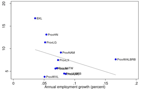
Figure A2. Average unemployment rates and employment growth across Belgian provinces, 2003-2015
Source:Calculations using Compensation NUTS2 regions. See section A.1. of the appendix for more information on the data.
A.6. PVAR ESTIMATION AND METHODOLOGY
The estimation method follows the works of Love and Zicchino (2006), and Abrigo and Love (2015) who discuss model selection and estimation of PVARs in a generalized method of moments (GMM) framework. As Love and Zicchino (2006) explain it, the PVAR methodology combines the traditional VAR approach by treating all variables in the system as endogenous, with the panel-data approach which allows for unobserved individual heterogeneity. An important consideration when estimating PVARs however, is that fixed-effects are correlated with the regressors of the lags of the dependent variables, as described by Nickell (1981). In order to account for this bias, two different methods are used in the literature today when estimating PVARs. The first method consists in performing the Helmert transformation which takes into account fixed effects by demeaning the variables, thereby attenuating the Nickell bias (Arellano and Bover, 1995). The second method controls for this bias by using lagged regressors as instruments, and estimates the coefficients by system GMM (Love and Zicchino, 2006). This
BXL
ProvANTW ProvHN
ProvLG
ProvLX
ProvLim ProvNAM
ProvOVL ProvVLBRB
ProvWALBRB
ProvWVL
5
10
15
20
0 .05 .1 .15 .2
36
paper uses the former method, however, the results obtained using the latter method are consistent with the findings.
A.7. EQUIVALENCE OF RELATIVE EMPLOYMENT RATE AND RELATIVE UNEMPLOYMENT RATE
In this paper, the responses of relative employment rates are shown. The multiple papers in the literature using the same model of estimation vary in the use of relative employment rate or relative unemployment rate. The choice of the one or the other is equivalent, as shown by Decressin and Fatas (1995):
𝑛𝑖𝑡 = log(𝑁𝑖𝑡) − log(𝑁𝑏𝑡) (11) Where 𝑁𝑖𝑡 is the employment rate (employment divided by labor force) in province i at time t, and 𝑁𝑏𝑡 is the employment rate of Belgium. Since log(𝑁𝑖𝑡) ≈ −𝑈𝑖𝑡, the above expression is equivalent to
𝑢𝑖𝑡 = 𝑈𝑖𝑡 − 𝑈𝑏𝑡 (12) Where 𝑈𝑖𝑡 is the unemployment rate (unemployment divided by labor force) in province i at time t, and 𝑈𝑏𝑡 is the unemployment rate of Belgium. The results obtained for the relative employment rate can thus be analyzed as the negative of relative unemployment rates, as defined above.
A.8. CONFIDENCE INTERVALS: RELATIVE EMPLOYMENT GROWTH - RELATIVE EMPLOYMENT RATE - RELATIVE PARTICIPATION RATE
37
Figure A3. Impulse Responses of Relative Employment Growth (a), Relative Employment Rate (b), and Relative Participation Rate (c)
-0.006 -0.005 -0.004 -0.003 -0.002 -0.001 0 0.001 0.002
0 1 2 3 4 5 6 7 8 9 10
(a)
95% confidence interval Relative Employment Growth
-0.006 -0.004 -0.002 0 0.002 0.004
0 1 2 3 4 5 6 7 8 9 10
(b)
95% confidence interval Relative Employment rate
-0.006 -0.004 -0.002 0 0.002 0.004 0.006 0.008
0 1 2 3 4 5 6 7 8 9 10
(c)
38
A.9. ESTIMATION: RELATIVE EMPLOYMENT - RELATIVE WAGE
This section provides the complete analysis of the joint movements of relative
employment rates and relative wages to a shock in labor demand.
If relative wages adjusted very strongly to the demand shock, this might provide
incentives for job creation (in-migration of firms), and thus reduce the impact of the initial shock
and the need for migration of workers. The estimation is performed by looking at the joint
behavior of relative employment growth and relative wages with the following PVAR model:
∆𝑒𝑖𝑡 = 𝛼𝑖10+ 𝛼𝑖11(𝐿)∆𝑒𝑖,𝑡−1+ 𝛼𝑖12(𝐿)𝑤𝑖,𝑡−1+ 𝜀𝑖𝑒𝑡 (13) 𝑤𝑖𝑡 = 𝛼𝑖10+ 𝛼𝑖11(𝐿)∆𝑒𝑖𝑡+ 𝛼𝑖12(𝐿)𝑤𝑖,𝑡−1+ 𝜀𝑖𝑤𝑡 (14) Where all the variables are defined as before and 𝑤𝑖𝑡 is the difference between the logarithm of wage in province i at time t minus its aggregated value for Belgium. Two lags are included in the model and the estimation is done by pooling all provinces together, allowing for fixed-effects. Once the PVAR model is computed, the impulse responses are derived, with the shock in relative employment growth defined as before as being 𝜀𝑖𝑒.
Firgure A4. Response of Relative Employment and Relative Wages to a Relative Employment shock
Source: Calculations based on System. The shock is -1 standard deviation to relative employment. Confidence intervals are
provided below.
-0.008 -0.007 -0.006 -0.005 -0.004 -0.003 -0.002 -0.001 0
39
The results show that the response of relative employment is almost identical to the one
obtained earlier. Furthermore, relative wages show a very small response to the shock, quickly
decreasing and returning to zero. Thus relative wages seem to exhibit a rather small role in the
adjustment process, very similar to the one observed for the relative employment rate.
The confidence intervals are obtained by running 200 Monte Carlo simulations using Gaussian approximation. While the confidence intervals seem to give high confidence in the results obtained for relative employment growth, some caution is needed when looking at the response of relative wages.
Figure A5. Impulse Responses of Relative Employment Growth (d), and Relative Wage (e)
-0.006 -0.005 -0.004 -0.003 -0.002 -0.001 0 0.001
0 2 4 6 8 10 12 14 16 18 20
(d)
95% confidence interval Relative Employment Growth
-0.004 -0.003 -0.002 -0.001 0 0.001
0 2 4 6 8 10 12 14 16 18 20
(e)