www.biogeosciences.net/4/87/2007/ © Author(s) 2007. This work is licensed under a Creative Commons License.
Biogeosciences
Marine geochemical data assimilation in an efficient Earth System
Model of global biogeochemical cycling
A. Ridgwell1, J. C. Hargreaves2, N. R. Edwards3, J. D. Annan2, T. M. Lenton4, R. Marsh5, A. Yool5, and A. Watson4 1School of Geographical Sciences, University of Bristol, Bristol, UK
2Frontier Research Center for Global Change, 3173-25 Showa-machi, Kanazawa-ku, Yokohama, Kanagawa 236-0001, Japan 3Earth Sciences, The Open University, Walton Hall, Milton Keynes, UK
4School of Environmental Sciences, University of East Anglia, Norwich, UK
5National Oceanography Centre, Southampton, European Way, Southampton SO14 3ZH, UK Received: 17 July 2006 – Published in Biogeosciences Discuss.: 10 August 2006
Revised: 13 December 2006 – Accepted: 15 January 2007 – Published: 25 January 2007
Abstract.We have extended the 3-D ocean based “Grid EN-abled Integrated Earth system model” (GENIE-1) to help un-derstand the role of ocean biogeochemistry and marine sedi-ments in the long-term (∼100 to 100 000 year) regulation of atmospheric CO2, and the importance of feedbacks between CO2and climate. Here we describe the ocean carbon cycle, which in its first incarnation is based around a simple single nutrient (phosphate) control on biological productivity. The addition of calcium carbonate preservation in deep-sea sedi-ments and its role in regulating atmospheric CO2is presented elsewhere (Ridgwell and Hargreaves, 2007).
We have calibrated the model parameters controlling ocean carbon cycling in GENIE-1 by assimilating 3-D obser-vational datasets of phosphate and alkalinity using an ensem-ble Kalman filter method. The calibrated (mean) model pre-dicts a global export production of particulate organic carbon (POC) of 8.9 PgC yr−1, and reproduces the main features of dissolved oxygen distributions in the ocean. For estimating biogenic calcium carbonate (CaCO3) production, we have devised a parameterization in which the CaCO3:POC export ratio is related directly to ambient saturation state. Calibrated global CaCO3 export production (1.2 PgC yr−1)is close to recent marine carbonate budget estimates.
The GENIE-1 Earth system model is capable of simulat-ing a wide variety of dissolved and isotopic species of rele-vance to the study of modern global biogeochemical cycles as well as past global environmental changes recorded in pa-leoceanographic proxies. Importantly, even with 12 active biogeochemical tracers in the ocean and including the calcu-lation of feedbacks between atmospheric CO2 and climate, we achieve better than 1000 years per (2.4 GHz) CPU hour on a desktop PC. The GENIE-1 model thus provides a viable Correspondence to:A. Ridgwell
alternative to box and zonally-averaged models for studying global biogeochemical cycling over all but the very longest (>1 000 000 year) time-scales.
1 Introduction
The societal importance of better understanding the role of the ocean in regulating atmospheric CO2 (and climate) is unquestionable. Reorganizations of ocean circulation and nutrient cycling as well as changes in biological produc-tivity and surface temperatures all modulate the concentra-tion of CO2in the atmosphere, and are likely central to ex-plaining the observed variability in CO2 over the glacial-interglacial cycles of the past∼800 000 years (Siegenthaler et al., 2005). These same marine carbon cycle processes will also affect the uptake of fossil fuel CO2in the future. Inter-actions between marine biogeochemistry and deep-sea sedi-ments together with imbalances induced between terrestrial weathering and the sedimentary burial of calcium carbonate (CaCO3)exert further controls on atmospheric CO2(Archer et al., 1998). These sedimentation and weathering processes are suspected to have dominated the recovery of the Earth system from catastrophic CO2release in the geological past (Zachos et al., 2005), and will largely determine the long-term future fate of fossil fuel CO2(Archer et al., 1998).
Understanding how atmospheric CO2is regulated thus nec-essarily requires feedbacks between CO2and climate to be taken into account. Coupled GCM ocean-atmosphere plus carbon cycle models (e.g., “HadCM3LC”; Cox et al., 2000) are important tools for assessing climate change and associ-ated feedbacks over the next few hundred years. However, their computational demands currently make them unsuit-able for investigating time-scales beyond 1000 years or for conducting sensitivity studies. So-called “off-line” carbon cycle models in which the ocean circulation has been pre-calculated such as the off-line tracer transport HAMOCC3 model of Maier-Reimer (1993) are much faster. However, the fixed circulation field employed in these models means that the importance of feedbacks with climate cannot easily be explored, except in a highly parameterized manner (Archer et al., 2004; Archer, 2005).
In contrast, marine biogeochemical box models, which consider the global ocean in terms of relatively few (typi-cally between about 3 and about 12) distinct volumes (the “boxes”), are extremely computationally efficient. Models of this type have an illustrious pedigree (e.g., Sarmiento and Toggweiler, 1984; Broecker and Peng, 1986) and continue today to be the tools of choice for many questions involv-ing processes operatinvolv-ing on time-scales of∼10,000 years or longer such as those involving ocean-sediment interactions and weathering feedbacks (e.g., Zeebe and Westbroek, 2003; Ridgwell, 2005; Yool and Tyrrell, 2005). Box models are also important tools in situations where the inherent uncer-tainties are large and need to be extensively explored (e.g., Parekh et al., 2004). Box models, as with GCMs, have spe-cific limitations. Validation against marine observations and sediment records is problematic because large volumes of the ocean are homogenized in creating each “box”, whereas biogeochemical processes are extremely heterogeneous both within ocean basins as well as between them. It is also difficult to incorporate a responsive climate or circulation, which is why box models are in effect off-line tracer trans-port models. The coupled meridional box model of Gildor et al. (2002) is one exception to this. Concerns have also been recently raised regarding whether box models present an inherently biased picture of certain aspects of the oceanic control of atmospheric CO2(Archer et al., 2003).
This has led to the development of fast climate models with reduced spatial resolution and/or more highly param-eterized “physics” – known variously as Earth System (Cli-mate) Models (ESMs) (Weaver et al., 2001) and Earth Sys-tem Models of Intermediate Complexity (EMICs) (Claussen et al., 2002). While ESMs have been instrumental in helping address a range of carbon cycling and climate change ques-tions, we believe that they have yet to realize their full po-tential. In particular, simulations on the time-scale of ocean-sediment interaction (order 10 000 years) are still relatively computationally expensive in many ESMs based around 3-D ocean circulation models, whereas in faster “2.5-3-D” mod-els (e.g., Marchal et al., 1998) the zonal averaging of the
basins complicates comparison between model and paleo-ceanographic data (Ridgwell, 2001).
In this paper we present a representation of marine bio-geochemical cycling within a 3-D ocean based Earth system model, which we calibrate for the modern carbon cycle via a novel assimilation of marine geochemical data. In a further extension to the model we describe the addition of carbon-ate preservation and burial in deep sea sediments (Ridgwell and Hargreaves, 2007). Together, these developments allow us to explore important questions surrounding future fossil fuel CO2uptake by the ocean and including the role of major feedbacks with climate (Ridgwell et al., 2006). However, as we discuss later, the initial biogeochemical modelling frame-work has important gaps, particularly with respect to the lack of a multi-nutrient description of biological productivity. There is also no representation of organic carbon burial or of suboxic diagenesis and the sedimentary control on ocean phosphate, nitrate, and sulphate concentrations. Continuing developments to this model will progressively address these areas and enable more extreme environmental conditions and events occurring earlier in Earth history to be explicitly as-sessed.
This paper is laid out as follows: we first describe the ocean biogeochemistry model itself (Sect. 2), then how the model is calibrated by assimilating observed marine geo-chemical data (Sect. 3). In Sect. 4 we present the predictions of the model for modern marine biogeochemical cycling, and discuss the specific limitations of very low resolution 3-D ocean circulation models such as we use here. We conclude in Sect. 5, summarising the pros and cons of the model as well as outlining the future development path.
2 Description of the “GENIE-1” model
The basis of our work is the fast climate model of Edwards and Marsh (2005) (“C-GOLDSTEIN”), which features a re-duced physics (frictional geostrophic) 3-D ocean circula-tion model coupled to a 2-D energy-moisture balance model (EMBM) of the atmosphere and a dynamic-thermodynamic sea-ice model (see Edwards and Marsh, 2005, for a full de-scription). The ocean model used here is non-seasonally forced and implemented on a 36×36 equal-area horizontal grid, comprising 10◦increments in longitude but uniform in
sine of latitude, giving∼3.2◦ latitudinal increments at the
equator increasing to 19.2◦in the highest latitude band. The
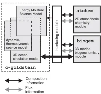
ocean has 8z-coordinate levels in the vertical. The grid and bathymetry is shown in Fig. 1.
-240 -180 -120 -60 90
0 60
Depth (km) 0
-90
0 1 2 3 4 5 6
Fig. 1.Gridded continental configuration and ocean bathymetry of the 8-level, 36×36 equal-area grid version of the GENIE-1 model.
as well as their molar relationships (if any) to sedimentary solids and atmospheric gases. For this present study, we se-lect only: total dissolved inorganic carbon (DIC), alkalinity (ALK), phosphate (PO4), oxygen (O2), 11 and CFC-12, the carbon and phosphorus components of dissolved or-ganic matter, plus the stable (13C) and radio- (14C) isotope abundances associated with both DIC and dissolved organic carbon. The circulation model thus acts on the 3-D spatial distribution of a total of 14 tracers including temperature and salinity.
As with many ocean circulation models, C-GOLDSTEIN employs a rigid lid surface boundary condition: i.e., grid cell volumes are not allowed to change. Net precipitation-minus-evaporation (P-E) at the ocean surface is then implemented as a virtual salinity flux rather than an actual loss or gain of freshwater. The concentration of biogeochemical tracers (DIC, ALK, PO4, etc.) should respond similarly to salinity: becoming more concentrated or dilute depending on the sign of P-E. To achieve this, one could apply virtual fluxes of the biogeochemical tracers along with salinity to the ocean sur-face (e.g., see the OCMIP-2 protocol; Najjar and Orr, 1999). We take the alternative approach here, and salinity-normalize the biogeochemical tracer concentration field prior to the cal-culation of ocean transport (Marchal et al., 1998). Once the ocean transport of tracers has been calculated, the salinity-normalized field is converted back to actual tracer concen-trations and a re-scaling of biogeochemical tracer concentra-tions carried out to ensure that there has been no gain or loss of biogeochemical tracers from the ocean as a whole as a result of the salinity transformations. The effects of biologi-cal uptake and remineralization and air-sea gas exchange are then calculated.
We have developed a representation of marine biogeo-chemical cycling called BIOGEM (for: BIOGEobiogeo-chemical Model) that calculates the redistribution of tracer
concen-atchem
biogem
Composition information Flux information
2D atmospheric chemistry module
3D marine biogeochemistry module 3D ocean
circulation model
dynamic-thermodynamic sea-ice model
Energy Moisture Balance Model
interfacing
module
c-goldstein
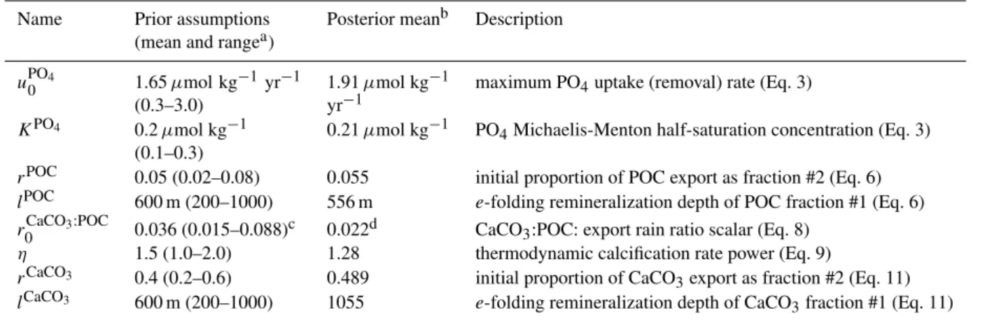
Fig. 2. Schematic of the relationship between the different model components comprising GENIE-1. Arrows represent the coupling of compositional information (black) and fluxes (grey). The bold highlights indicate the biogeochemical extensions to the climate model (C-GOLDSTEIN) (Edwards and Marsh, 2005) that are de-scribed in this paper. The current implementation of the module ATCHEM (not described in the text) is rather trivial – it consists of a 2-D 36×36 atmospheric grid storing atmospheric composi-tion, together with a routine to homogenize composition across the grid each time-step. The efficient numerical terrestrial scheme ENTS and modifications to the EMBM described in Williamson et al. (2006) are not used in this study, so that the land surface is es-sentially passive.
trations occurring other than by transport by the circulation of the ocean. This happens through the removal from so-lution of nutrients (PO4)together with DIC and ALK, by biological activity in the sunlit surface ocean layer (the eu-photic zone), which has a depth ofhe=175 m in the 8-level ocean model configuration. The resulting export of partic-ulate matter to the ocean interior is subject to “remineral-ization” – the metabolic and dissolution processes that re-lease constituent species back into inorganic solution, but at greater depth compared to the level at which the tracers were originally removed from solution. Further redistribution of tracers occurs through gas exchange with the atmosphere as well as due to the creation and destruction of dissolved or-ganic matter. BIOGEM has a conceptual relationship with the climate model as shown schematically in Fig. 2. We refer to the overall composite model as GENIE-1.
length as the ocean (0.01 yr), even in response to rather ex-treme (15 000 PgC) releases of (fossil fuel) CO2to the atmo-sphere.
2.1 Ocean biogeochemical cycling
The low vertical resolution of the ocean circulation model and need to maximize computational speed for long simu-lations and sensitivity analyses dictates that the “biological” part of the marine carbon cycle be relatively abstracted. A more important reason for starting off with as simple a de-scription of surface biological productivity as possible is to reduce the number of free parameters in the model which must be optimized, particularly since this work represents the first attempt to assimilate marine geochemical observa-tions within a prognostic 3-D circulation model of the ocean. Of course, as the nature of the assimilation problem becomes better defined and the capabilities and limitations of available optimization techniques better understood, we expect to sub-sequently re-calibrate the marine carbon cycle in conjunction with increasingly sophisticated multiple-nutrient biological schemes.
In this paper we estimate new (export) production directly from available surface nutrient concentrations, a robust tac-tic used in many early ocean carbon cycle models. In other words, what we have is “conceptually not a model of biol-ogy in the ocean but rather a model of biogenically induced chemical fluxes (from the surface ocean)” (Maier-Reimer, 1993). Overall, the biological export scheme is function-ally similar to that of Parekh et al. (2005), and we adopt their notation where relevant. The main difference is that we currently consider only a single nutrient, phosphate (PO4), rather than co-limitation with iron (Fe).
The governing equations in BIOGEM for the changes in phosphate and dissolved organic phosphorus (DOP) concen-trations occurring in the surface ocean layer (but omitting the extra transport terms that are calculated by the ocean circu-lation model; Edwards and Marsh, 2005) are:
∂PO4
∂t = −Ŵ+λDOP (1)
∂DOP
∂t =νŴ−λDOP (2)
Ŵ=uPO4
0 ·
PO4
PO4+KPO4 ·(1−A)·
I
I0
(3) whereŴ is the biological uptake of PO4. Ŵ is calculated from: (i)uPO4
0 , an assumed maximum uptake rate of phos-phate (mol PO4 kg−1 yr−1) that would occur in the ab-sence of any limitation on phytoplankton growth, and (ii) a Michaelis-Menten type kinetic limitation of nutrient uptake, of whichKPO4 is the half-saturation constant. Because of the degree of abstraction of ecosystem function inherent in our model, the appropriate values for eitheruPO4
0 or KPO4 are
not obvious, and so are subsequently calibrated (see Sect. 3 and Table 1). We apply two modifiers on productivity rep-resenting the effects of sub-optimal ambient light levels and the fractional sea ice coverage of each grid cell (A)(Edwards and Marsh, 2005). A full treatment of the effects of light lim-itation on phytoplankton growth is beyond the scope of this current paper. The strength of local insolation (I )is there-fore simply normalized to the solar constant (I0)to give a limitation term that is linear in annual incident insolation. A proportion (ν)of PO4 taken up by the biota is partitioned into dissolved organic phosphorus (DOP). The relatively la-bile dissolved organic molecules are subsequently reminer-alization with a time constant of 1/λ. The values ofν and
λare assigned following the assumptions of the OCMIP-2 protocol (Najjar and Orr, 1999):ν=0.66 andλ=0.5 yr−1.
The particulate organic matter fraction is exported verti-cally and without lateral advection out of the surface ocean layer at the next model time-step. Because there is no explicit standing plankton biomass in the model, the export flux of particulate organic phosphorus (FzPOP=he, in units of mol PO4 m−2yr−1)is equated directly with PO4uptake (Eq. 1):
FzPOP=h
e =
Z 0
he
ρ·(1−ν)·Ŵ dz (4)
whereρ is the density of seawater andhe the thickness of the euphotic zone (175 m in the 8-level version of this ocean model).
In the production of organic matter, dissolved inorganic carbon (DIC) is taken out of solution in a 106:1 molar ratio with PO4(Redfield et al., 1963) while O2takes a−170:1 ra-tio with PO4(Anderson and Sarmiento, 1994). The effect on total alkalinity (ALK) of the biological uptake and remineral-ization of nitrate (NO3)is accounted for via a modification of ALK in a−1:1 ratio with the quantity of NO3transformed. Because we do not model the nitrogen cycle explicitly in this paper, we link ALK directly to PO4 uptake and rem-ineralization through the canonical 16:1 N:P ratio (Redfield et al., 1963). For convenience, we will describe the various transformations involving organic matter in terms of carbon (rather than phosphorus) units, the relationship between or-ganic matter export fluxes being simply:
FzPOC=he =106·FzPOP=he (5)
We represent the remineralization of particulate organic car-bon (POC) as a process occurring instantaneously through-out the water column. We partition POC into two distinct fractions with different fates in the water column, following Ridgwell (2001) but adopting an exponential decay as an al-ternative to a power law. The POC flux at depthzin the water column is:
FzPOC=FzPOC=h
e·
1−rPOC+rPOC·exp
z
he−z
lPOC
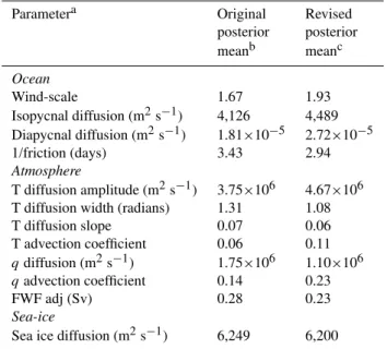
Table 1.EnKF calibrated biogeochemical parameters in the GENIE-1 model.
Name Prior assumptions (mean and rangea)
Posterior meanb Description
uPO4
0 1.65µmol kg
−1yr−1
(0.3–3.0)
1.91µmol kg−1 yr−1
maximum PO4uptake (removal) rate (Eq. 3)
KPO4 0.2µmol kg−1 (0.1–0.3)
0.21µmol kg−1 PO4Michaelis-Menton half-saturation concentration (Eq. 3)
rPOC 0.05 (0.02–0.08) 0.055 initial proportion of POC export as fraction #2 (Eq. 6) lPOC 600 m (200–1000) 556 m e-folding remineralization depth of POC fraction #1 (Eq. 6) rCaCO3:POC
0 0.036 (0.015–0.088)c 0.022d CaCO3:POC: export rain ratio scalar (Eq. 8)
η 1.5 (1.0–2.0) 1.28 thermodynamic calcification rate power (Eq. 9)
rCaCO3 0.4 (0.2–0.6) 0.489 initial proportion of CaCO
3export as fraction #2 (Eq. 11)
lCaCO3 600 m (200–1000) 1055 e-folding remineralization depth of CaCO
3fraction #1 (Eq. 11)
athe range is quoted as 1 standard deviation either side of the mean bquoted as the mean of the entire EnKF ensemble
cassimilation was carried out on a log 10scale
dNote that the rain ratio scalar parameter is not the same as the CaCO
3:POC export rain ratio as measured at the base of the euphotic zone, becauserCaCO3:POC
0 is further multiplied by (−1)ηto calculate the rain ratio, whereis the surface ocean saturation state with respect to calcite (see Sect. 2.1). Pre-industrial mean ocean surfaceis∼5.2 in the GENIE-1 model, so that the global CaCO3:POC export rain ratio can be estimated using the 8-parameter assimilation as being equal to (5.2–1)1.28×0.022=0.14.
(Table 1). Because we explicitly resolve the individual “com-ponents” (i.e., C,13C, P, . . . ) of organic matter, the GENIE-1 model can be used to quantify the effect of fractionation between the components of organic matter during remineral-ization (e.g., Shaffer et al., 1999) as well as between differ-ent carbon isotopes. However, we assume no fractionation during remineralization in this present study. The residual flux of particulate organic material escaping remineralization within the water column is remineralized at the ocean floor, making the ocean-atmosphere system closed with respect to these tracers (i.e., there is no loss or gain to the system).
The modern ocean is oxic everywhere at the resolution of our model (e.g., see Fig. 6). However, O2 availability may be insufficient under different ocean circulation regimes and continental configurations. To broaden the applicability of the GENIE-1 model to past climates and biogeochemi-cal cycling, we limit remineralization according to the to-tal availability of electron acceptors – if dissolved O2 is depleted and NO3 is selected as an active tracer in the model, denitrification occurs to provide the necessary ox-idant: 2NO−3→N2+3O2. If NO−3 becomes depleted and SO24− has been selected as an active tracer, sulphate re-duction occurs: 2H++SO24−→H2S+2O2. If the total con-centration of selected electron-accepting tracer species (O2, NO3, SO4)is still insufficient, remineralization of POC is restricted. Our strategy thus differs from other modeling ap-proaches in which remineralization always strictly conforms to a predetermined profile and the consequences of excess oxidation over O2availability are resolved either by numer-ically preventing negative oxygen concentrations occurring
(e.g. Zhang et al., 2001, 2003) or by allowing the tracer transport of negative O2concentrations (e.g., Hotinski et al., 2001). We treat the remineralization of dissolved organic matter in an analogous manner if O2 availability is insuffi-cient.
H2S created through sulphate reduction is oxidized in the presence of O2at a rate (mM H2S h−1):
d[H2S]
dt=k· [H2S] · [O2]2 (7)
where [H2S] and [O2] are the dissolved concentra-tions of hydrogen sulphide and oxygen, respectively, and
k=0.625 mM−2h−1(Zhang and Millero, 1993).
well as explicitly simulating sulphate reduction and sulphide release to the ocean, which currently we treat implicitly as a water-column process in order to avoid problems en-countered in previous models when O2 demand due to or-ganic matter remineralisation exceeds dissolved O2 availabil-ity (Hotinski et al., 2001; Zhang et al., 2001, 2003).
Open ocean dwelling calcifying plankton such as coc-colithophorids and foraminifera produce calcium carbonate (CaCO3) in addition to organic compounds (see Ridgwell and Zeebe, 2005, for a review of the global carbonate cycle). As the ecological processes which regulate calcifier activity are not well understood, early models incorporating marine carbonate production calculated the export flux of CaCO3 in a fixed production ratio with POC (e.g., Broecker and Peng, 1986; Yamanaka and Tajika, 1996). Derivatives of this approach modify the CaCO3:POC rain ratio as some func-tion of temperature (e.g., Marchal et al., 1998) and/or opal flux (e.g., Heinze et al., 1999; Archer et al., 2000; Heinze, 2004). Current ecosystem models include a measure of com-petition between calcifying phytoplankton such as coccol-ithophores and non-calcifying ones such as diatoms to es-timate CaCO3production (e.g., Moore et al., 2002; Bopp et al., 2003). However, there are drawbacks with this strategy because there are doubts as to whether autotrophic coccol-ithophorids are the dominant source of CaCO3 in the open ocean (Schiebel, 2002), or whether Emiliania huxleyi is a sufficiently representative species of global coccolith carbon-ate production to be chosen as the functional type calcifying species in ecosystem models (Ridgwell et al., 2006).
Recent work has introduced a further dimension as to how CaCO3production should be represented in models. Exper-iments have shown that planktic calcifiers such as coccol-ithophores (Riebesell et al., 2000; Zondervan et al., 2001; Delille et al., 2005) and foramifera (Bijma et al., 1999) pro-duce less carbonate at lower ambient carbonate ion concen-trations (CO23−). A progressive reduction in surface CO23− is an expected consequence of fossil fuel invasion into the ocean (Kleypas et al., 1999; Caldeira and Wickett, 2003; Freely et al., 2004; Orr et al., 2005). Several recent studies have incorporated a response of the CaCO3:POC rain ratio to changes in surface ocean carbonate chemistry, by employing a parameterization based on the deviation from modern sur-face ocean conditions of either CO2partial pressure (Heinze, 2004) or CO23− (Barker et al., 2003). We present a new approach here, one which relates the export flux of CaCO3 (FCaCO3
z=he )to the POC flux (F POC
z=he)via a thermodynamically-based description of carbonate precipitation rate:
FCaCO3
z=he =γ·r
CaCO3:POC
0 ·F
POC
z=he (8)
whererCaCO3:POC
0 is a spatially-uniform scalar, and γ is a thermodynamically-based local modifier of the rate of car-bonate production (and thus of the CaCO3:POC rain ratio), defined:
γ =(−1)η >1.0 (9a)
γ =0.0 ≤1.0 (9b)
whereηis a constant andis the ambient surface satura-tion state (solubility ratio) with respect to calcite, defined by the ratio of the product of calcium ion (Ca2+)and carbonate
ion (CO23−)concentrations toKSP, the solubility constant (Zeebe and Wolf-Gladrow, 2001):
=[Ca
2+
][CO23−]
KSP
(10)
In formulating this parameterization we have drawn on de-scriptions of abiotic carbonate system dynamics in which the experimentally observed precipitation rate can be linked to saturation via an equation with the same form as Eq. (9) (e.g., Burton and Walter, 1987). What this equation says is that the precipitation rate increases with a greater ambi-ent environmambi-ental degree of supersaturation with respect to the solid carbonate phase (>1.0), with the power parame-terηcontroling how non-linear the response of calcification is. At ambient saturation states below the point of thermody-namic equilibrium (=1.0) (“undersaturation”) no carbonate production occurs. It should be noted that although coccol-ithophorid and foraminiferal calcification rates are observed to respond to changes in saturation (e.g., Bijma et al., 1999; Riebesell et al., 2000; Zondervan et al., 2001; Delille et al., 2005), we do not explicitly capture other important controls. Instead, we have implicitly collapsed the (poorly understood) ecological and physical oceanographic controls on carbonate production onto a single, purely thermodynamic dependence on.
For this paper we take our prior assumptions regarding the suspected values of η (Table 1) from previous analysis of neritic (shallow water) calcification (Opdyke and Wilkinson, 1993; Zeebe and Westbroek, 2003; Ridgwell, 2004; Langdon and Atkinson, 2005). Elsewhere we collate available obser-vational data on pelagic calcifiers and explore the effect of alternative prior assumptions inη(Ridgwell et al., 2006).
The remineralization (dissolution) of CaCO3 in the wa-ter column is treated in a similar manner to particulate or-ganic carbon (the parameter nomenclature being analogous to Eq. 6):
FCaCO3
z =
FCaCO3
z=he ·
1−rCaCO3+rCaCO3·exp
z
he−z
lCaCO3
(11)
2.2 Air-sea gas exchange
The flux of gases (mol m−2yr−1)across the air-sea interface is given by:
F =k·ρ·(Cw−α·Ca)·(1−A) (12)
wherekis the gas transfer velocity (m yr−1),ρ the density of sea-water (kg m−3), Cw the concentration of the gas dis-solved in the surface ocean (mol kg−1), C
athe concentration of the gas in the overlying atmosphere (atm), andAthe frac-tional ice-covered area. The parameterαis the solubility co-efficient (mol kg−1atm−1)and is calculated from the coeffi-cients listed by Wanninkhof (1992) (and references therein). Gas transfer velocities are calculated as a function of wind speed following Wanninkhof (1992):
k=a·u2·(Sc/660)−0.5 (13)
whereuis the annual mean climatological wind speed andSc
is the Schmidt Number for the specific gas following Wan-ninkhof (1992) (and references therein). We use the scalar annual average wind speed field of Trenberth et al. (1989) for calculating air-sea gas exchange and set the scaling constant
a=0.31 (Wanninkhof, 1992), which gives us a global annual mean gas transfer coefficient for CO2equal to 0.058 mol m−2 yr−1µatm−1in the calibrated model (Sect. 3.2).
For completeness, we include the parameterization of air-sea gas exchange for all the gases listed by Wanninkhof (1992) although this calculation is not made if the relevant dissolved tracers in the ocean and/or atmosphere are not se-lected. To facilitate analysis of the biogeochemical conse-quences of anoxia and the existence of a sulphidic ocean at times in the geologic past, we also allow for the exchange of H2S, for which we take the solubility following Millero (1986) and Schmidt number from Khalil and Rasmussen (1998).
2.3 Isotopic tracers and fractionation
Fractionation occurs between12C and13C during the biolog-ical fixation of dissolved carbon (as CO2(aq))to form organic and inorganic (carbonate) carbon, as well as during air-sea gas exchange. For the production of organic carbon (both as POC and DOC) we adopt the fractionation scheme of Ridg-well (2001):
δ13CPOC=δ13CCO2(aq)−ε
f + εf−εd·
KQ
[CO2(aq)]
(14)
whereδ13CCO2(aq) and [CO2
(aq)] are the isotopic composi-tion and concentracomposi-tion of CO2(aq), respectively. εf andεd are fractionation factors associated with enzymic intercellu-lar carbon fixation and CO2(aq) diffusion, respectively, and assigned values ofεf=25‰ andεd=0.7‰ (Rau et al., 1996,
1997). KQ is an empirical approximation of the model of Rau et al. (1996, 1997) as described by Ridgwell (2001):
KQ=2.829×10⁻¹⁰−1.788×10⁻⁷·T+3.170×10⁻⁵·T2 (15)
withT the ocean temperature in Kelvin.
For CaCO3, we adopt a temperature-dependent fractiona-tion for calcite following Mook (1986). The air-sea13C/12C fractionation scheme follows that of Marchal et al. (1998), with the individual fractionation factors all taken from Zhang et al. (1995). Solution of the isotopic partitioning of car-bon between the different aqueous carcar-bonate species (i.e., CO2(aq), HCO−2, CO
2−
3 )follows Zeebe and Wolf-Gladrow (2001).
For radiocarbon, the14C/12C fractionation factors are sim-ply the square of the factors calculated for13C/12C at every step. Radiocarbon abundance also decays with a half-life of 5730 years (Stuiver and Polach, 1977). We report radiocar-bon isotopic properties in the114C notation, which we cal-culate directly from model-simulatedδ13C andδ14C values by:
114C=1000·
1+
δ14C
1000
!
· 0.975
2
1+δ100013C
2−1
(16)
which is the exact form of the more commonly used ap-proximation:114C=δ14C−2· δ13C+25
· 1+δ14C/1000
(Stuiver and Polach, 1977). δ14C is calculated us-ing δ14C= AS/Aabs−1
·1000, where AS is the (model-simulated) sample activity and Aabsis the absolute interna-tional standard activity, related to the activity of the oxalic acid standard (AOx)by Aabs=0.95·AOx. AOx is assigned a ratio of 1.176×10⁻¹²(Key et al., 2004).
2.4 Definition of the aqueous carbonate system
The aqueous carbonate chemistry scheme used in the calibra-tion is that of Ridgwell (2001). In this, alkalinity is defined following Dickson (1981) but excluding the effect of NH3, HS−, and S2−. The set of carbonate dissociation constants
are those of Mehrbach et al. (1973), as refitted by Dick-son and Millero (1987), with pH calculated on the seawa-terpH scale (pHSWS). Numerical solution of the system is via an implicit iterative method, seeded with the hydrogen ion concentration ([H+]) calculated from the previous
time-step (Ridgwell, 2001) (or with 10−7.8 from a “cold” start). We judge the system to be sufficiently converged when [H+]
changes by less than 0.1% between iterations, which typi-cally occurs after just 2 or 3 iterations. This bringspH and
fCO2to within±0.001 units (pHSWS) and±0.2µatm, re-spectively, compared to calculations made using the model of Lewis and Wallace (1998).
explicitly. Here, we do not select them, and instead estimate their concentrations from salinity (Millero, 1982, 1995) in order to solve the aqueous carbonate system. Furthermore, because we do not consider the marine cycling of silicic acid (H4SiO4)here we implicitly assume a zero concentration ev-erywhere. The error in atmospheric CO2induced by this sim-plification compared to prescribing observed concentrations of H4SiO4(Conkright et al., 2002) in the model is<1µatm. Subsequent to the EnKF calibration presented here, refine-ments have been made to the representation of aqueous car-bonate chemistry in the GENIE-1 model including a more comprehensive definition of alkalinity – still following Dick-son (1981) but now the only exclusion being the contribution from S2−. The set of carbonate dissociation constants re-main those of Mehrbach et al. (1973) (refitted by Dickson and Millero, 1987), the apparent ionization constant of water follows Millero (1992), andpH is calculated on the seawater
pH scale: otherwise, all other dissociation constants and as-sumptions follow those adopted in Zeebe and Wolf-Gladrow (2001). The impact of these model parameterization changes has only a very minor impact on the marine carbon cycle: equivalent to a reduction in mean ocean DIC of <1µmol kg−1with atmospheric CO2 held constant at 278 ppm (see Sect. 4.1).
3 Data assimilation and calibration of the marine car-bon cycle
The degree of spatial and temporal abstraction inherent in representations of complex global biogeochemical processes inevitably gives rise to important parameters whose values are not well known a priori. Because of the computational cost of most 3-D ocean biogeochemical models, calibration of the poorly known parameters usually proceeds by trial-and-error with the aid of limited sensitivity analysis. The relative speed of the GENIE-1 model allows us to explore a new efficient and optimal approach to this problem by assim-ilating 3-D fields of marine geochemical data using a version of the ensemble Kalman filter which has been developed to simultaneously estimate multiple parameters in climate mod-els.
In the following sections it should be noted that the ensem-ble Kalman filter (EnKF) methodology is described in detail in Annan et al. (2005a) where it is applied to identical twin testing of the GENIE-1 climate model as proof-of-concept for the technique. Subsequent application of the EnKF to op-timization of the climate component of the GENIE-1 model is described in Hargreaves et al. (2004). Here we simply ap-ply the same EnKF methodology to the ocean biogeochem-istry as was performed in this previous calibration of the model climatology.
3.1 EnKF methodology
The model parameters were optimized with respect to 3-D data fields that are available for the present day climatologi-cal distributions of phosphate (PO4)(Conkright et al., 2002) and alkalinity (ALK) (Key et al., 2004) in the ocean. The data were assimilated into the model using an iterative application of the ensemble Kalman filter (EnKF), which is described more fully in Annan et al. (2005a, b). The EnKF was orig-inally introduced as a state estimation algorithm (Evensen, 1994). We introduce the parameters into the analysis simply by augmenting the model state with them. The EnKF solves the Kalman equation for optimal linear estimation by using the ensemble statistics to define the mean and covariance of the model’s probability distribution function. In other words, the resulting ensemble members are random samples from this probability distribution function. Although this method is only formally optimal in the case of a linear model and an infinite ensemble size, it has been shown to work well in cases similar to ours (Hargreaves et al., 2004; Annan et al., 2005a).
The parameter estimation problem studied here is a steady state problem, somewhat different in detail (and in princi-ple simprinci-pler) than the more conventional time-varying imprinci-ple- imple-mentations of the EnKF. However, the prior assumption of substantial ignorance, combined with the nonlinearity of the model and high dimensionality of the parameter space be-ing explored, means that a direct solution of the steady state problem does not work well. Therefore, an iterative scheme has been developed which repeats a cycle of ensemble infla-tion, data assimilation and model integration over a specified time interval, in order to converge to the final solution. (See the references mentioned above for the technical details.) As demonstrated in Annan et al. (2005a) and Annan and Har-greaves (2004), this iterative method converges robustly to the correct solution in identical twin testing. Further applica-tions using real data have also been successful with a range of different models (e.g., Hargreaves et al., 2004; Annan et al., 2005b, c). The method is relatively efficient, requiring a total of approximately 100 times the equilibrium time of the model to converge, and it is exact in the case of a linear model and a large ensemble size.
As mentioned above, the EnKF ensemble randomly sam-ples the probability distribution function defined by the model, data and prior assumptions. Therefore, the ensem-ble members do not themselves converge to the optimum but instead sample the region around it, with the ensemble mean being a good estimate of the optimum. Where all uncertain-ties are well defined, the spread of the ensemble members indicates the uncertainty surrounding this optimum. How-ever, this is not the case here, since many model parame-terizations are poorly understood and may be inadequate in various ways. A good example is the uncertainty surround-ing the role of dust and the marine iron cycle (Jickells et al., 2005). The formulation of the biogeochemical model is thus inherently more uncertain than that of a physical model, and, at this stage, there is no clear way to estimate the true uncer-tainty of the calibrated model. We therefore use the EnKF to produce a single calibrated model version, taking the mean of this ensemble as an estimate of the best parameters.
The marine carbon cycle is calibrated against long-term average observations of PO4 (Conkright et al., 2002) and ALK (Key et al., 2004) distributions in the ocean. We chose these data targets on the basis that PO4will help constrain the cycling of organic matter within the ocean, while ALK will (primarily) help constrain the cycling of CaCO3in the ocean. We assume that their observed distributions are relatively un-affected by anthropogenic change (Orr et al., 2005) (although see Feely et al., 2004). To create the PO4and ALK assimila-tion targets, we transformed the 3-D data-sets of Conkright et al. (2002) and Key et al. (2004), respectively, to the GENIE-1 model grid, and salinity-normalized the data. For the surface data target, although the model surface layer is 175 m thick, the observed data is integrated only over the uppermost 75 m for calculating surface boundary conditions – the depth as-sumed in the OCMIP-2 protocol as the nominal consump-tion depth separating the producconsump-tion zone (above) from the consumption zone (below) (Najjar and Orr, 1999).
The calibration of the biogeochemistry used an ensemble size of 54, which was chosen primarily for computational convenience. Ocean chemistry was initialized with uniform concentrations of: 2244µmol kg−1 DIC (estimated pre-Industrial) (Key et al., 2000), 2363µmol kg−1ALK (Key et al., 2000), 2.159µmol kg−1PO3−
4 (Conkright et al., 2001), and 169.6µmol kg−1 O2 (Conkright et al., 2002). Initial concentrations of dissolved organic matter are zero, as are
δ13C andδ14C. AtmosphericpO2was initially set at 0.2095 atm and allowed to evolve freely in response to net air-sea gas exchange thereafter. Atmospheric CO2was continually restored to a value of 278 ppm throughout the assimilation. The parameters we considered in the EnKF assimilation as well as our prior assumptions regarding their likely values are listed in Table 1.
Table 2. EnKF calibrated climate parameters in the GENIE-1 model.
Parametera Original Revised
posterior posterior
meanb meanc
Ocean
Wind-scale 1.67 1.93
Isopycnal diffusion (m2s−1) 4,126 4,489 Diapycnal diffusion (m2s−1) 1.81×10⁻⁵ 2.72×10⁻⁵
1/friction (days) 3.43 2.94
Atmosphere
T diffusion amplitude (m2s−1) 3.75×10⁶ 4.67×10⁶ T diffusion width (radians) 1.31 1.08
T diffusion slope 0.07 0.06
T advection coefficient 0.06 0.11
qdiffusion (m2s−1) 1.75×10⁶ 1.10×10⁶
qadvection coefficient 0.14 0.23
FWF adj (Sv) 0.28 0.23
Sea-ice
Sea ice diffusion (m2s−1) 6,249 6,200
asee Edwards and Marsh (2005) and Lenton et al. (2006) bHargreaves et al. (2004)
cparameter values employed here (re-calibrated as per Hargreaves
et al., 2004, but using a corrected equation of state – see Sect. 3.1)
3.2 Results of the EnKF assimilation
The mean and standard deviation of the ensemble values of the controlling biogeochemistry parameters are listed in Ta-ble 1. Most of the parameters showed only weak correla-tions in the posterior ensemble, with the striking exception ofrCaCO3:POC
0 andη, as shown in Fig. 4. We can trace this relationship back to Eqs. (8) and (9), where it implies that
rCaCO3:POC
0 ·(−1)
ηis close to being constant. We interpret this to mean that although total global production of carbon-ate is relatively tightly constrained by the data, the spatial variation, which is a function of local saturation state ()in the model, is not as well constrained.
Depth
(km)
0 1 2 3 4 5
0.0
Depth
(km)
0 1 2 3 4 5
0
-90 -60 -30 30 60 90-90 -60 -30 0 30 -90 -60 -30 0 30 60 90
DA
T
A:
A
TL.
DA
T
A:
IND.
DA
T
A:
P
AC.
MODEL:
A
TL.
MODEL:
IND.
MODEL:
P
AC.
Depth
(km)
0 1 2 3 4 5
Depth
(km)
0 1 2 3 4 5
0
-90 -60 -30 30 60 90-90 -60 -30 0 30 -90 -60 -30 0 30 60 90
DA
T
A:
A
TL.
DA
T
A:
IND.
DA
T
A:
P
AC.
MODEL:
A
TL.
MODEL:
IND.
MODEL:
P
AC.
1.0 2.0 3.0
2250 2300 2350 2400 2450
PO
(
mol
kg
)
4
m
-1
ALK
(
mol
kg
)
m
-1
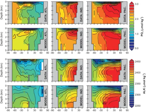
Fig. 3.Data assimilation of PO4and ALK. The top panel shows the basin averaged meridional-depth distribution of phosphate (PO4), with the model simulation immediately below the respective observations (Conkright et al., 2002). The bottom panel shows the basin averaged meridional-depth distributions of alkalinty (ALK) (Key et al., 2004). Note that we plot this data as actual concentrations, whereas the assimilation is carried out on salinity-normalized values.
data set to the model output. We interpret this in terms of the interpolation procedure used by Key et al. (2004) producing a more self-consistent data-set compared to the empirically based reconstruction of Goyet et al. (2000).
Analysis of ocean respiration patterns led Andersson et al. (2004) to propose a double exponential as a useful de-scription for the profile of POC flux with depth. We tested a parameterization for the remineralization of POC in which each of the two fractions was assigned a characteristic (expo-nential decay) length scale. The mean EnKF calibrated rem-ineralization length scales were 96 m and 994 m, compared to values of 55 m and ∼2200 m determined by Andersson et al. (2004). However, the coarse vertical resolution of the model employed here means that we cannot place any con-fidence in length scales shorter than a few hundred meters. The improved fit to upper ocean PO4gradients using a dou-ble exponential in the EnKF comes at the expense of a rather negligible POC flux to the ocean floor because of the poor data constraint provided by the relatively weak gradients of PO4in the deep ocean (e.g., see Fig. 3).
Achieving an appropriate particulate flux to the ocean floor is critical to the determination of sedimentary carbonate con-tent and organic carbon burial (see: Ridgwell and Harg-reaves, 2007). We therefore retain the Eq. (6) parameteriza-tion in which one of the fracparameteriza-tions has a fixed and effectively infinite length scale. An identical assumption of exponential
decay combined with a recalcitrant fraction was employed in the sediment trap analysis of Lutz et al. (2002). Although they found considerable regional variations in vertical trans-port, the mean fraction of POC export reaching the abyssal ocean in their analysis was 5.7%, which is almost identical to our EnKF calibrated value of 0.055 (5.5%) for parameter
rPOC (Table 1). Furthermore, the mean depth scale of de-cay of the remaining 94.3% of exported POC was found to be 317 m (Lutz et al., 2002), which while somewhat shorter than our calibrated value of 556 m (parameterlPOC)is of the same order. Thus, independent analysis of annual POC sink-ing fluxes is largely consistent with our inverse modellsink-ing of global PO4distributions, particularly at depth. We believe that further improvement, particularly to the shallow length-scale will be possible within the context of an ocean circula-tion model with higher vertical resolucircula-tion (e.g., 16 levels).
4 Discussion
4.1 The calibrated baseline state of the model
0.0
h
0.5 1.0 1.5 2.0 2.5
-3.0 -2.5 -2.0 -1.5
log
(
)
10
0
r
CaCO3:POC
R = 0.95
2Fig. 4. Relationship between the parameters controlling CaCO3 production. The values ofrCaCO3:POC
0 andη(Eq. 8) are plotted for all 54 ensemble members (crosses), as well as the best-fit relation-ship between them (solid line): log10rCaCO3:POC
0
=−0.6564·
η−1.2963.
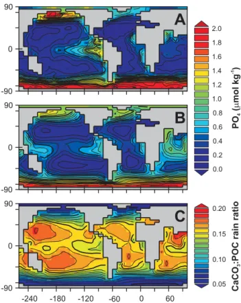
with the observations to a first-order (Conkright et al., 2002), with relatively high (>0.5µmol kg−1)concentrations in the Southern Ocean, North Pacific, North Atlantic, and Eastern Equatorial Pacific, and nutrient depletion (<0.5µmol kg−1) in the mid latitude gyres. However, over-estimated low lat-itude upwelling results in excess (>0.5µmol kg−1)PO4 in the Western Equatorial Pacific and Equatorial Indian Ocean. In addition, there is no representation of iron limitation, crit-ical in the modern ocean in restricting nutrient depletion in the “High Nutrient Low Chlorophyll” (HNLC) regions of the ocean such as the North and Eastern Equatorial Pacific, and Southern Ocean (Jickells et al., 2005). The calibration must then strike a compromise – PO4 uptake (scaled by the pa-rameter,uPO4
0 in Eq. 3) must be sufficiently low that nutri-ents remain unused in the HNLC regions, yet at the same time, high enough to deplete nutrients elsewhere. The re-sult is that PO4is generally slightly lower than observed in the HNLC regions but slightly too high elsewhere. However, overall, global export production of particulate organic car-bon (POC) is 8.91 GtC (PgC) yr−1, consistent with recent estimates (e.g., Amount et al., 2003; Schmittner et al., 2005; Jin et al., 2006).
The lack of an explicit representation of iron limitation in conjunction with the simplistic treatment of light limitation is an obvious deficiency in this initial incarnation of the marine biogeochemical model. Despite this, the general structure of PO4 is still reasonably reproduced. Thus, we would argue that the single nutrient (PO4)limitation scheme is adequate for developing and exploring geochemical assimilation tech-niques such as the EnKF.
For alkalinity (ALK), we achieve a generally reason-able simile of the zonally-averaged distributions in each ocean basin (Fig. 3). The main areas of model-data mis-match concern surface concentrations. These are
primar--240 -180 -120 -60
-90 90
0 0
60
0.05 0.10 0.20
0.15
-90 90
0
-90 90
0
0.2 0.4 0.6 0.8 1.0 1.2 1.6
1.4 1.8 2.0
0.0
A
B
C
Fig. 5. Surface ocean properties. (A)Observed PO4 concentra-tions in the surface ocean (integrated over the uppermost 75 m) (Conkright et al., 2002) compared to the model surface layer pre-dictions(B).(C)The predicted distribution of CaCO3:POC export ratio.
Depth
(km)
0
1
2
3
4
5
0
Depth
(km)
0
1
2
3
4
5
0
-90 -60 -30 30 60 90-90 -60 -30 0 30 -90 -60 -30 0 30 60 90
DA
T
A:
A
TL.
DA
T
A:
IND.
DA
T
A:
P
AC.
MODEL:
A
TL.
MODEL:
IND.
MODEL:
P
AC. 100
200 300
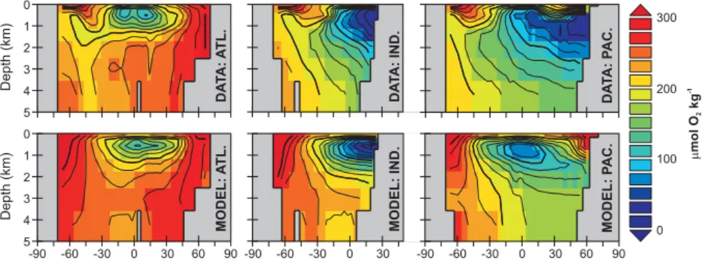
Fig. 6.Basin averaged meridional-depth distributions of dissolved oxygen in the ocean: observed (top) (Conkright et al., 2002) and model-simulated for the year 1994 (bottom).
With a mean ocean ALK of 2363µmol kg−1(Key et al., 2004), a (pre-Industrial) atmospheric CO2concentration of 278 ppm requires a mean ocean DIC of 2214µmol kg−1 compared to an observationally-based estimate of 2244µmol kg−1(Key et al., 2004). Some 14µmol kg−1of this apparent DIC difference is explained by mean surface alkalinity being slightly lower than observed (2301µmol kg−1compared to an average of 2310µmol kg−1 over the uppermost 75 m of the modern ocean (Conkright et al., 2002), itself mainly a consequence of the low surface salinities simulated by the climate model (particularly in the Atlantic) (Hargreaves et al., 2004). Use of a revised “Redfield ratio” value of 1:117 linking phosphorus and carbon in organic matter (Ander-son and Sarmiento, 1994) increases DIC by∼7µmol kg−1, while using observed ocean surface temperatures (in place of climate model simulated temperatures) in the calculation of air-sea gas exchange accounts for another 2µmol kg−1 DIC. The residual model-data difference (9µmol kg−1DIC) is comparable to the uncertainty in the GLODAP data-sets of
∼5–10µmol kg−1(Key et al., 2004). However, we cannot rule out convective ventilation or insufficient sea-ice extent in the Southern Ocean, lack of seasonality, and/or the thickness of the model surface ocean layer, contributing to driving the DIC inventory slightly too low (see discussion in Sect. 4.3). 4.2 The marine biogeochemical cycling of O2
The model reproduces the main features of the observed dis-tribution of dissolved oxygen (O2)in the ocean (Fig. 6), with elevated concentrations associated with the sinking and sub-duction of cold and highly oxygenated waters in the North Atlantic, as well as the occurrence of intermediate depth min-ima at low latitudes in all three ocean basins. Deep ocean O2concentrations are almost everywhere correct to within
∼40µmol kg−1of observations (Conkright et al., 2002). The area of greatest model-data mismatch concerns the ventila-tion of intermediate waters in the Southern Ocean and North Pacific. In addition, while the magnitude of O2depletion of the oxygen minimum zone in the northern Indian Ocean is
correctly predicted, it lies at too shallow a depth and is too restricted in vertical extent. Overall, however, the quality of our O2simulation compares favorably with predictions made by considerably more computationally expensive ocean cir-culation models (e.g., Bopp et al., 2002; Meissner et al., 2005).
4.3 Ocean circulation and biogeochemical cycling in very coarse resolution models
While large-scale heat transports in the ocean are well cap-tured (Hargreaves et al., 2004), the steady-state distribution of dissolved oxygen (Fig. 6) highlights the excess ventila-tion of intermediate depths above ca. 1500 m in parts of the Southern Ocean and North Pacific in the GENIE-1 model. We can demonstrate that ocean transport rather than pro-cesses associated with organic production and/or remineral-ization is primarily responsible by simulating the transient uptake of CFC-11 and CFC-12 from the atmosphere. We use a similar methodology to OCMIP-2 (Dutay et al., 2002), in which the partial pressure of CFCs in the atmosphere follow observations for the years 1932 to 1998 (Walker et al., 2000) and with air-sea gas exchange calculated explicitly accord-ing to Eqs. (12) and (13). The model-predicted 1994 global ocean CFC-11 inventory is 0.88×10⁹mol, compared to the observationally-based estimate of 0.55±0.08×10⁹mol (Key et al., 2004; Willey et al., 2004), with Southern Ocean inter-mediate depths accounting for more than half of the model-data mismatch.
20 20
20 20
20
20
40
40 40
40 40
40
60 6080
40 40
40 40
40
40 40
40
40 40
40
40 8080
80 -90
90
0
-240 -180 -120 -60 -90
90
0 0
60
0 10 20 30 40 50 60 70 80
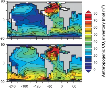
Fig. 7. Water column integrated anthropogenic CO2inventory in the ocean for the year 1994: observed (top) (Key et al., 2004) and model-simulated (bottom).
of intermediate waters in the North (East) Pacific and par-ticularly in the Southern Ocean where the excess (compared to observations) South of 41◦S is 21 PgC. The main areas of anthropogenic CO2 model-data mismatch are similar to those of CFC-11 and are also consistent with the locations of excess O2concentrations in the model – see Fig. 6. How-ever, subduction of anthropogenically CO2enriched water to depth in the North Atlantic is well reproduced in addition to there being a reasonable match to the observations at low and mid latitudes.
There may be a fundamental limitation as to how coarse a resolution a 3-D ocean circulation model may have and still be able to simulate decadal-scale uptake processes ac-curately. This is because the stability of the water column at high latitudes appears to be very sensitive to the vertical resolution. For instance, it has recently been demonstrated (M¨uller et al., 2006) that a signification improvement in tran-sient tracer uptake is obtained in a very similar ocean GCM to that used here by increasing the number of vertical lev-els from 8 to 32, although the use of observed climatological surface boundary conditions and separation of eddy-induced and isopycnal mixing effects may also have been critical in this. We have investigated this further by repeating the OCMIP-2 transient tests with 16 rather than 8 levels in the ocean (Edwards and Marsh, 2005) and find that the radio-carbon properties of the deep ocean indeed become much closer to the observations, with model-predicted114C val-ues below 2000 m in the Southern Ocean of ca.−140‰ and ca.−200‰ in the North Pacific.
Thus, simply increasing the vertical resolution appears to be an effective strategy in creating a more stable water col-umn at high latitudes. However, this comes at a
compu-year 250
300 350 400 450 500 550 600
0 100 200 300 400 500 600 700 800 900 1000
0.1 1.0 10 100 1000
250 300 350 400 450 500 550 600
Fig. 8. Ocean CO2invasion behavior. Predicted evolution of at-mospheric CO2following an instantaneous doubling to 556 ppm. The atmospheric CO2behavior of GENIE-1 is consistent with the four ocean carbon cycle models which ran this experiment out as part of OCMIP-2 (Doney et al., 2004). The OCMIP-2 models are those of: Stocker et al. (1992), Yamanaka and Tajika (1996), Gor-don et al. (2000), and Schlitzer (2002). We deliberately do not dif-ferentiate between the different OCMIP-2 models here to highlight the comparison between GENIE-1 and models having much greater horizontal and/or vertical resolution, rather than discuss the reasons for the differences amongst the OCMIP-2 models. All OCMIP-2 trajectories are therefore plotted as identical grey lines. The 8-level version of GENIE-1 is shown as a thin solid black line, while the improvement in decadal-scale CO2uptake resulting from doubling the vertical resolution is illustrated by the thin dashed black line. The bottom plot shows the same data, but plotted on a logarithmic time axis to help visually separate out the different time-scales of CO2invasion.
tational price because there is an approximate doubling of the number of cells in the ocean. To address century to millennial-scale (and longer) questions, particularly those in-volving interaction with deep-sea sediments we retain the 8-level ocean by default, but recognize the limitations we have identified in 8-level vs. 16-levels in representing some decadal (and sub-decadal) processes.
3-D structure of PO4 and ALK in the ocean, global export would have to be similarly overestimated. In contrast, as noted in Sect. 4.1, the diagnosed export of POC lies towards the centre of the spread of current (high resolution) GCM es-timates while the estimated global export flux of CaCO3is near identical to the recent GCM data- assimilation study of Jin et al. (2006), itself one of the lowest values for CaCO3 export flux proposed. In addition, the mean fraction of ex-ported POC reaching the deep ocean as well as the shallower remineralisation length-scale diagnosed from sediment trap analysis (Lutz et al., 2002) are consistent with our inverse-modelled parameter values (Sect. 3.2).
We confirm our assumptions regarding the century-scale (and beyond) applicability of an 8-level configuration by run-ning an OCMIP-2 test, in which an abiotic ocean is brought to steady state with an atmospheric CO2 concentration of 278 ppm, atmospheric CO2instantaneously doubled, and the invasion of CO2into the ocean then tracked for 1000 years (Orr, 2002). We find that atmospheric CO2 concentrations diverge between our 8-level model and the OCMIP-2 models over the first few decades of uptake, but the trajectories re-converge thereafter (Fig. 8), making the century-scale (and longer) CO2behavior in GENIE-1 indistinguishable from the differing OCMIP-2 model behaviors. This is consistent with simulations we have made of radiocarbon distributions in the ocean (not shown) in which predicted (natural)114C prop-erties of deep ocean water masses also fall within the range of OCMIP-2 model behavior (Matsumoto et al., 2004). That we reproduce the year 2100 prediction for the strength of “CO2-calcification” feedback (the enhancement of CO2 up-take from the atmosphere due to reduced calcification) made by a much higher resolution ocean model (Ridgwell et al., 2006) also supports our assertion regarding the time-scales of applicability of the fast 8-level version of the GENIE-1 model.
5 Conclusions and perspectives
We have constructed a 3-D ocean based Earth System Model that includes key feedbacks between marine carbon cycling, atmospheric CO2, and climate, yet even when simulating 12 biogeochemical tracers in the ocean together with the ex-change with the atmosphere of 6 gaseous tracers, achieves better than 1000 yr simulated per (2.4 GHz) CPU hour on a desktop computer. The computational speed of the GENIE-1 model has enabled us to calibrate via an Ensemble Kalman Filter (EnKF) method the critical parameters controlling ma-rine carbon cycling. The EnKF has also allowed us to judge the consistency of available global alkalinity data-sets with our mechanistic representation of global biogeochemical cy-cling, and has determined the a priori unknown relationship between η andrCaCO3:POC
0 in our parameterization of bonate production. Overall, global particulate organic car-bon and inorganic (carcar-bonate) carcar-bon export predicted by the
calibrated model is consistent with recent data- and model-based estimates and despite the very coarse resolution of the ocean model, the distribution of dissolved O2 in the ocean generally compares favorably with the data and with the re-sults of much more computationally expensive 3-D ocean cir-culation models.
However, important caveats are raised by our analysis re-garding very low resolution configurations of the GENIE-1 model. As highlighted by the results of the OCMIP-2 tests presented in Sect. 4.3, the transient tracers (CFCs, anthro-pogenic CO2, and bomb114C) delineate apparent deficien-cies in the ventilation of intermediate waters in the Southern Ocean and North Pacific. This means that estimates made by this version of the model of the anthropogenic CO2 uptake by the ocean on time-scales much shorter than∼100 years should be treated with caution. We find that an increased number of vertical levels produces a signification improve-ment in simulated transient tracer behaviour, suggesting that there is a limit to how low the vertical resolution of a GCM may be and yet still maintain adequate water column stability everywhere. Because our results highlight the importance of global biogeochemical cycling in providing a sensitive diag-nostic of ocean circulation in models, we propose that more physically realistic models might be achieved by “co-tuning” key physical and biogeochemical parameters.
A second caveat concerns our highly-parameterized sin-gle nutrient (PO4)scheme for marine biological production. While this simple scheme gave us important advantages in developing the EnKF calibration of the model against global biogeochemical observations, it has the obvious disadvan-tage that there is no representation of iron limitation, which is critical in the modern ocean in restricting nutrient deple-tion in the HNLC regions of the ocean such as the North and Eastern Equatorial Pacific, and Southern Ocean. The con-sequence of this is that the overall quality of fitting of global PO4distributions in the EnKF is somewhat degraded because the appropriate mechanism for achieving relatively high PO4 in the HNLC regions is absent. This will be addressed in the first instance by incorporating the biogeochemical scheme and Fe cycle of Parekh et al. (2005) into the GENIE-1 model. Further planned developments will include an optional func-tional type ecosystem model as well as the addition of the limiting nutrients nitrate and silicic acid.
diagenesis following Archer et al. (2002) and the regenera-tion of phosphate from anoxic sediments.
Finally, although the particular configuration of the GENIE-1 model presented here is extremely fast compared to other coupled and even off-line GCMs models of ocean carbon cycling, it is still too numerically expensive to en-able application to >1 Myr time-scales. Box models will this remain essential tools for addressing the very longest time-scale questions. However, the speed and multi-tracer capabilities make the GENIE-1 model a viable alternative to marine biogeochemical box models for questions regarding the controls on atmospheric CO2on∼100 to multi 100 000 year time-scales.
Acknowledgements. A. Ridgwell acknowledges a University Re-search Fellowship from the Royal Society as well as support from Canada Research Chairs and the Canadian Foundation for Climate and Atmospheric Sciences. Development of the model was sup-ported by the NERC e-Science programme (NER/T/S/2002/00217) through the Grid ENabled Integrated Earth system modelling (GE-NIE) project (http://www.genie.ac.uk) and by the Tyndall Centre for Climate Change Research (Project TC IT 1.31). Computer fa-cilities for the EnKF calculations were provided by JAMSTEC. We are indebted to the generosity of OCMIP-2 participants who made their unpublished model CO2results available to us: A. Ishida and Y. Yamanaka at the Frontier Research Center for Global Change, Japan (formerly “IGCR”), F. Joos at Climate and Environmental Physics, Bern, and R. Schlitzer of AWI-Bremerhaven.
Edited by: T. W. Lyons
References
Anderson, L. and Sarmiento, J.: Redfield ratios of remineralization determined by nutrient data analysis, Global Biogeochem. Cy-cles, 8, 65–80, doi:10.1029/93GB03318, 1994.
Andersson, J. H., Wijsman, J. W. M., Herman, P. M. J., et al.: Respiration patterns in the deep ocean, Geophys. Res. Lett., 31, L03304, doi:10.1029/2003GL018756, 2004.
Annan, J. D. and Hargreaves, J. C.: Efficient parameter estimation for a highly chaotic system, Tellus A, 56, 520–526, 2004. Annan, J. D., Hargreaves, J. C., Edwards, N. R., and Marsh, R.:
Parameter estimation in an intermediate complexity Earth Sys-tem Model using an ensemble Kalman filter, Ocean Modell., 8, 135–154, 2005a.
Annan, J. D., Lunt, D. J., Hargreaves J. C., and Valdes, P. J.: Pa-rameter Nonlin. Processes Geophys., 12, 363–371, 2005b. Annan, J. D., Hargreaves, J. C., Ohgaito, R., Abe-Ouchi, A., and
Emori, S.: Efficiently constraining climate sensitivity with en-sembles of paleoclimate simulations, SOLA, 1, 181–184, 2005c. Archer, D.: Modeling the calcite lysocline, J. Geophys. Res., 96,
17 037–17 050, 1991.
Archer, D., Kheshgi, H., and Maier-Reimer, E.: Dynamics of fossil fuel CO2neutralization by marine CaCO3, Global Biogeochem. Cycles, 12, 259–276, 1998.
Archer, D., Winguth, A., Lea, D., and Mahowald, N.: What caused the glacial/interglacial atmospheric pCO2 cycles?, Rev. Geo-phys., 38, 159–189, 2000.
Archer, D. E., Morford, J. L., and Emerson, S. R.: A model of suboxic sedimentary diagenesis suitable for automatic tuning and gridded global domains, Global Biogeochem. Cycles, 16, doi:10.1029/2000GB001288, 2002.
Archer, D. E., Martin, P. A., Milovich, J., Brovkin, V., Plattner, G.-K., and Ashendel, C.: Model sensitivity in the effect of Antarctic sea ice and stratification on atmosphericpCO2, Paleoceanogra-phy, 18, 1012, doi:10.1029/2002PA000760, 2003.
Archer, D., Martin, P., Buffet, B., et al.: The importance of ocean temperature to global biogeochemistry, Eeart Plant. Sci. Lett., 222, 333–348, 2004.
Archer, D.: Fate of fossil fuel CO2in geologic time, J. Geophys. Res., 110, C09S05, doi:10.1029/2004JC002625, 2005.
Aumont, O., Maier-Reimer, E., Blain, S., and Monfray, P.: An ecosystem model of the global ocean including Fe, Si, P colimitations, Global Biogeochem. Cycles, 17, 1060, doi:10.1029/2001GB001745, 2003.
Barker, S., Higgins, J. A., and Elderfield, H.: The future of the car-bon cycle: review, calcification response, ballast and feedback on atmospheric CO2, Philosophical Trans. Royal Soc. A, 361(30), 1977–1999, 2003.
Bijma, J., Spero, H. J., and Lea, D. W.: Reassessing foraminiferal stable isotope geochemistry: Impact of the oceanic carbonate system (Experimental Results), in: Use of proxies in paleo-ceanography: Examples from the South Atlantic, edited by: Fis-cher, G. and Wefer, G., 1339 Springer-Verlag Berlin Heidelberg, 489–512, 1999.
Bopp, L., LeQu´er´e, C., Heimann, M., Manning, A. C., and Monfray, P.: Climate-induced oceanic oxygen fluxes: Implications for the contemporary carbon budget, Global Biogeochem. Cycles, 16, 1022, doi:10.1029/2001GB001445, 2002.
Bopp, L., Kohfeld, K. E., Le Quere, C., and Aumont, O.: Dust impact on marine biota and atmospheric CO2during glacial pe-riods, Paleoceanography, 18, 1046, doi:10.1029/2002PA000810, 2003.
Broecker, W. S. and Peng, T.-H.: Glacial to interglacial changes in the operation of the global carbon cycle, Radiocarbon, 28, 309– 327, 1986.
Burton, E. A. and Walter, L. M.: Relative precipitation rates of arag-onite and Mg calcite from seawater – Temperature or carbonate ion control, Geology, 15, 111–114, 1987.
Caldeira, K. and Wickett, M. E.: Anthropogenic carbon and ocean pH, Nature, 425, 365, 2003.
Cameron, D. R., Lenton, T. M., Ridgwell, A. J., Shepherd, J. G., Marsh, R. J., and the GENIE team: A factorial analysis of the marine carbon cycle controls on atmospheric CO2, Global Biogeochem. Cycles, 19, GB4027, doi:10.1029/2005GB002489, 2005.
Claussen, M., Mysak, L. A., Weaver, A. J., et al.: Earth system models of intermediate complexity: closing the gap in the spec-trum of climate system models, Climate Dyamics., 18, 579–586, 2002.
Conkright, M. E., Antonov, J. I., Baranov, O. K., et al.: World Ocean Database 2001, Volume 1: Introduction, edited by: Lev-itus, S., NOAA Atlas, NESDIS 42, U.S. Government Printing Office, Washington, D.C., 167 pp, 2002.