Characterisation of S185 steel under monotonic loading by a feature tracking method

ABSTRACT

In this work, the mechanical behaviour of S185 steel under monotonic loading was characterised by using an image feature-based tracking method. Tensile tests on three types of cylindrical specimens were carried out, in particularly using smooth and notched specimens. Target features were painted on the specimen surfaces and tracked in images sequences in order to estimate the experimental load-displacement curves. Finite element analyses of the non-linear behaviour of steel components were also performed, being the parameters of the different plasticity employed determined by fitting the experimental and numerical data.

INTRODUCTION

Monotonic fracture on steel components can occur due to extreme loading conditions as support settlements, industrial plant shutdown and accidental loads. For ductile or plastic monotonic fracture, several models have been proposed as, for instance, empirical models, void growth models, porosity-type models and continuum damage mechanics (CDM) based models (Coppola, 2009). In this work, the models proposed by Gurson-Tvergaard-Needleman (Gurson, 1976; Tvergaard, 1984), Johnson-Cook (Johnson, 1985) and Kanvinde-Deierlein (Kanvinde, 2007) were used for modelling monotonic loading. The constitutive parameters of these models need to be estimated from suitable experimental approaches. Tensile tests coupled with an image-based feature tracking method (Xavier, 2009) were used to estimate the load-displacement material response.

Smooth (CL), large notch (CES) and small notch (CE) cylindrical specimens were machined from a S185 structural steel plate. These specimens were tested on a servo hydraulic INSTRON 8801 universal testing machine at room temperature. Circular marks were painted on the surface of the specimens and tracked in the images acquired during the tests at an acquisition frequency of 1 Hz. The image based tracking was done using a computational algorithm that allows the measurement of the displacements of the target features in a sequence of images acquired during the deformation of test sample. The load-displacement experimental curves obtained using the image tracking algorithm was used to calibrate the finite element models, which included a plasticity model with isotropic hardening. Numerical analyses using ANSYS® 12.1 (ANSYS, 2009) were conducted to compute the necessary parameters (stress-strain and triaxiality histories) to calibrate the Johnson-Cook (JC) and

PAPER REF: 2784

CHARACTERISATION OF S185 STEEL UNDER MONOTONIC

LOADING BY A FEATURE TRACKING METHOD

João Pereira1(*), Abílio de Jesus1, José Xavier2, João Manuel R.S. Tavares3

1

UCVE-IDMEC-LAETA/ Departamento de Engenharias, Escola de Ciências e Tecnologia da Universidade de Trás-os-Montes e Alto Douro, 5001-801 Vila Real, Portugal.

2

CITAB, University of Trás-os-Montes e Alto Douro, 5001-801 Vila Real, Portugal.

3

Departamento de Engenharia Mecânica, Faculdade de Engenharia Universidade do Porto / Instituto de Engenharia Mecânica e Gestão Industrial, Rua Dr. Roberto Frias, 4200-465 Porto, Portugal

(*)

MODELS FOR MONOTONIC DUCTILE FRACTURE

Johnson-Cook (JC) (Johnson-Cook, 1985), Gurson-Tvergaard-Needleman (GTN) (Gurson, 1976) and Kanvinde and Deierlein (KD) models were used in this study to predict the monotonic fracture in S185 structural steel components. In the present section, these models are introduced.

The JC model allows to obtain the ductile/damage curve and provides the relation between the equivalent strain at fracture and a monotonic function of the stress triaxiality (Wierzbicki, 2005), and can be expressed as follows:

 

1 2exp 3

f

ε C C C η (1)

where the stress triaxiality, η, is defined by the ratio between the hydrostatic pressure, p ,

and the Von Mises equivalent stress, σ_VM, as follows:

VM p η σ  (2) 1

C , C and ₂ C are constants that characterise the material and are determined using the ₃

monotonic tensile tests data, addressing distinct stress triaxialities and fracture strain. In this work, the JC model was calibrated by means of an experimental program of tensile tests performed in cylindrical specimens. The determination of the stress triaxiality in the critical region is complex, since it is variable during the loading process. To overcome this shortcoming the following equation was used:

 

_

where _f is the strain at fracture.

Regarding the GTN model, it assumes that the microdefects and microcavities in the material microstructure can be accountable during the damage evolution process due to an external load. Hence, this process is based on micromechanical assumptions as growth, nucleation and coalescence of voids inside the material. As such, failure occurs when the void volume fraction, f , reaches the critical value (Gurson, 1976):

0

V f

V

 (4)

where V represent the voids volume within an initial volume of material, V . ₀

According to the GTN model, the reduction of resistance is addressed by the introduction of the yield surface described by the plastic potential, F_Gurson, (Broggiato, 2007):

2

* 3 *2

1 2 cosh

eq p

where _s represent the current yield stress, _eq is the equivalent stressq , ₁ q are materials ₂

parameters related with the interaction of microvoids and the relationship 2 3 1

q q is assumed,

*

v

f is the effective void volume fraction defined as (Broggiato, 2007):





where f is the current void volume fraction, _v f and _C f are the failure porosity and critical _F

porosity respectively. The evolution of void volume fraction can be divided into two parts: void growth rate and the void nucleation rate:

2 (1 ) 1 exp 2 2      _{  }     _{  }       v g n p g v kk p p N v v N n N N f f f f f f f S S      (7) where p v

 represents the equivalent macroscopic plastic strain rate, f denotes the effective _N

particle of the void nucleation, _N is the mean void nucleation and S is the standard _N

deviation of the normal distribution (Broggiato, 2007).

An ultra-low-cycle fatigue model developed for fatigue life prediction was the Kanvinde and Deierlein (KD) model (Kanvinde, 2007). However this model proposed corresponds to a generalization of a model for monotonic ductile fracture. Metallic materials contain voids in their microstructures, which may grow under the action of plastic deformation. Race and Tracey (Kanvinde, 2007) reported that, for a single spherical void in an infinite continuum, the void growth rate can be described as:

/ exp(1.5 ) _P

dR RC  d (8)

where R represents the average radius, C is a material constant and dε is the incremental _P

plastic strain. Integrating Eq. (8) and assuming void growth to be the controlling parameter of the monotonic fracture, the failure criterion for monotonic damage may be expressed as:





0 exp 1.5

p _critical

monotonic p monotonic

VGI 



where VGI_monotonic is the void growth index, that is compared to a critical value, VGI_monotoniccritical . Thus, monotonic ductile fracture occurs when voids present in the material microstructure reaches the critical void growth index during the monotonic loading, as described by Eq. (9).

FEATURE TRACKING METHOD

In the framework of experimental solid mechanics, several interferometric and white-light optical methods have been proposed in the last decades for assessing the displacement or strain a region of interest (Rastogi, 2000; Grédiac, 2004). These techniques contrast with conventional strain gauges or extensometers by the fact that they provide full-field data and are contact-free. Among them, non-interferometric techniques, based on image and signal processing and analysis, have been increasingly used, such as the techniques of image correlation (Sutton, 2009; Pan, 2009), features tracking (Rotinat, 2001; Dahl, 2009) and grid (Surrel, 1996; Avril 2004). This class of techniques differs in terms of post-processing, but they share the same underlying principle of assessing the deformation of an object by analysing the geometrical deformation of a defined pattern, that assumed to be perfectly attached to the material surface under analysis. In the DIC method, the target surface has a random (speckle) texture pattern, which can exist naturally or be artificially defined using an aerosol spray or by airbrush painting. In the grid technique, a grid pattern (e.g., crossed vertical and horizontal lines) of a given pitch is transferred (glued) to the surface of interest. Both these techniques provide full-field displacements of a (quasi-) planar object and have been applied to a variety of mechanical and fracture problems, taking advantage of good balance between spatial resolution and resolution. However, there are certain case studies in which neither a random nor a periodic pattern can be conveniently defined on the surface under evaluation. This is the case, for instance, when wet specimens are used, or when the specimens have complex curved surfaces, or even when a very short period of time is available between the specimen preparation and testing. Moreover, when dealing with large deformation, either delamination of the painting used in the speckle pattern or significant grid pitch variation can occur when choosing the DIC or grid methods, respectively, making measurements unreliable. In such cases, an image feature-based tracking method can be a suitable alternative. This class of technique only requires few marks (local features) over the region of interest, which can be quickly transferred (painted) to a background surface. Normally, this technique does not have the same spatial resolution than counterpart DIC and grid methods, but can be suitable for measuring strains over uniform or moderate gradient fields (Dahl, 2009; Franke, 2007).

A feature tracking method was used in this work, based on algorithms of image processing and analysis (Xavier, 2009). In this method, it was assumed that: 1) few target points or features were defined on the surface of interest; 2) these marks follow the material deformation during the loading process. It should be noted that, for the purpose of this study, the low spatial resolution of this approach was not critical, since uniform strain/stress fields were expected over the regions of interest. Hence, this assessment image based technique relies on the tracking of the centroids of the target features. The strain state in the material can then be estimated by computing the change in the relative length among adjacent centroid occured during the deformation. Between the reference (0) and a given deformed configurations (t), the in-plane linear strains (_,0t with  1,2 directions) can be estimated by (Fig. 1a):





where Li_,i_,₀1_t represents the change of length between two adjacent centroids, Li_,i_,₀1 is the initial length in the reference state, and i1,,n_ 1 with n representing the total number _

of target features in the image along the  direction.

In order to solve Eq. (10), the in-plane coordinates of the centroids (x ) needed to be _

determined using techniques of image processing and analysis. The flowchart of the proposed tracking method is shown in Fig. 1b. In a first step, the images of the material sample under analysis have to be acquired before (0) and after (t), the deformation. A camera-lens optical system can be used aiming at a region of interest with suitable magnification. Usually, saturated images are acquired, in order to enhance the contrast between the target features (of black colour) and the uniform substratum of the material (of white colour). The acquired images can be cropped before the post-processing step so that a sub-image in which the target features are limited can be defined. Therefore, regions in the field of view outside the specimen under evaluation (typically, these regions correspond to dark zones of the surrounding environment or scene) are systematically eliminated. This step can be especeally advantageous in image segmentation and classification tasks, allowing a suitable definition of areas of both target features and scene background. A transformation of a grey level image, f(x,y), into the correspondent binary image, g(x,y), was then achieved by using a traditional thresholding algoritm with a suitable threshold value T. In the resultant binary image, the pixels labeled as 1 (one) correspond to target features, whilst pixels set to 0 (zero) are associated with image scene background. This classification is convenient for further image processing and analysis. Morphological operates were then applied to the binary images to eliminate some usually errors and imprecisions that occur in the detection of the target features over the region of interest: (i) the marks painted over the material surface can be imaged with a pronounced variation of light intensity distribution, from which it can be difficult to define a single closed region in the image segmentation step; (ii) natural spots of the material reflected over the surface of the specimen may be imaged with a grey level intensity closer to the one of the target features, resulting, after the segmentation, into a binary image with parasite stains over the region of interest. This image enhancement step consists in a combination of the erosion and dilation operations in order to completely fill and define the target features and/or remove the erroneous stain regions in the image background that persisted after the segmentation step. Finally, for each image, the total number of target features (n ) and their centroid locations (_ x ) are calculated. From the coordinates found, _

the distance between two adjacent centroids can then be determined as: i i i i x x L_,1 _1 _ (i1,,n_ 1) (11.a) and



Finally, the information resultant from the acquired images is used to solve Eq. (10) for yielding an estimation of the strain state on both 1(x) and 2(y) directions.

Image Crop: Region of interest Segmentation: Binary image Morphology: Target definition Analysis: Centroid calculation (a) (b)

Fig.1 (a) Schema of the target features; (b) Flowchart of the image feature-based tracking method used.

EXPERIMENTAL WORK Material and tested method

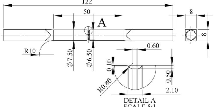
In order to identify the parameters of the models for monotonic ductile fracture proposed in this work, monotonic tensile tests were performed in three sets of smooth (CL) and notched (CE and CES) cylindrical specimens, which geometries are shown in Figure 2, 3 and 4, respectively. These specimens were extracted cut and then machined from a S185 structural steel plate with a thickness of 8mm. The monotonic tensile tests were carried out on a servo hydraulic INSTRON 8801 universal testing machine, at room temperature. A periodic pattern suitable for the image based tracking method used was painted in cylindrical specimens with a pitch of 5 mm, as illustrated in Figure 5. The processing of the images acquired during the tensile tests allowed obtaining the load-displacement experimental curves.

Fig 3. Geometry of the cylindrical specimens with small notch (CE) (dimensions in mm)

Fig 4. Geometry of cylindrical specimens with large notch (CES) (dimensions in mm)

1 ₂ 3

5 mm

Fig 5. Smooth cylindrical specimen (1) and notched cylindrical specimens with high (2) and low (3) notch severity.

The specimens were polished and painted using matte white aerosol spray for defining a uniform background pattern. Dark circular marks with about 2 mm in diameter were then pained on the specimen along the longitudinal direction as shown in Figure 5. These marks were spaced by 5 mm over the region of interest. Images were recorded by an 8-bit Baumer Optronic FWX20 digital camera (pixel resolution of 1624×1236 pixels) coupled with an Opto-Enginnering TC 23 36 telecentric lens (Table 1).This lens is more expensive and eventually larger and heavier than normal lenses of similar focal length, but can keep invariant the magnification factor of the optical system in a given working distance range. The lens aperture, the LED lighting intensity and the shutter time were set in order to achieve image saturation (i.e., pixel gray levels higher than 255 – 8 bits of resolution) for enhancing image contrast and therefore simplifying the image processing and analysis (Fig. 1b). Additionally, motion blur in the images during the exposure time when testing was prevented.

Table 1 Characteristics of the opto engineering telecentric lens TC 2336. Magnification 0.243 ± 3% Field of View (1/1.8”) 29.3 x 22.1 mm2 Working Distance 103.5 ± 2 mm Working F-number 8 Telecentricity < 0.08º Field Depth 11 mm

FINITE ELEMENT ANALYSES

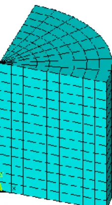
In order to access the parameters of JC and KD models numerical simulations were performed in ANSYS 12.1®. Three-dimensional models were built using the 8-node isoparametric solid element SOLID185 (ANSYS, 2009). Taking into account the axisymmetry of the specimens geometries only 1/ 4 of the geometry was used and the respective boundary conditions were applied. The finite element model of smooth cylindrical specimen is represented in Fig 6. The total length of the specimen model corresponds to the gauge length between two consecutive circular marks of the periodic pattern. For the notched specimens, the mesh of finite elements was built considering the periodic pattern suitable for the image tracking method application, as illustrate in Figures 7 and 8.

The finite element models include a plasticity model with isotropic hardening based on J2 yield criteria, which was fitted from load-displacement experimental curves. The true stress-strain curve introduced in finite element models is represented in Figure 9.

Fig 7. Finite element mesh of cylindrical specimen with small notch: a) overall view; b) limits of geometric model in accordance with the periodic pattern; c) detail mesh view.

Fig 8. Finite element mesh of the cylindrical specimen with small notch: a) overall view; b) limits of the geometric model in accordance with the periodic pattern; c) detailed mesh view.

0 100 200 300 400 500 600 700 800 St re ss [ M P a ] a) b) c) a) b) c)

Numerical simulations in ABAQUS 6.10®, were used to compute the parameters included in the porosity model proposed by Gurson, Tvergaard and Needleman. The geometries of the notched cylindrical specimens were also modelled in 3D three dimensions using the 8-node isoparametric solid element, C3D8R (ABAQUS, 2010). For the GTN model application the explicit analysis was used in ABAQUS® 6.10. Due to symmetry and axisymmetry conditions only 1/ 8 of a full scale model was used. To ensure the failure conditions of the specimens a remote displacement was applied. The finite element mesh of the notched specimens is illustrated in Figures 10 and 11.

The Gurson plasticity model included in the ABAQUS® library requires the definition of a hardening law. For this case the multilinear plasticity model with isotropic hardening fore mentioned was also used.

Fig 10. Finite element mesh of cylindrical speciemen with small notch (CE) built in ABAQUS® 6.10

Fig 11. Finite element mesh of cylindrical speciemen with large notch (CES) built in ABAQUS® 6.10

RESULTS AND DISCUSSION

In this section, the results obtained for the monotonic tensile tests of the cylindrical specimens are presented and discussed. The tracking method used in monotonic tensile allowed to determine the load-displacement experimental curves, which were correlated in order to calibrate the plasticity model with isotropic hardening used in the numerical simulations. Despite inability of the plasticity model to address the loss of strength at the failure instant, it allowed the characterization of the loss of load after the maximum force due to the non-linear behaviour compromised in the numerical analyses.

one curve. Taking into account that there is only a curve to describe the whole behaviour of the specimen and the compromise with another series of experimental results a satisfactory correlation was verified. The relative displacement was calculated based on the tracking the circular marks 2 and 3, Figure 12.

0 2 4 6 8 10 12 14 16 18 0 1 2 3 4 5 6 L oad [kN ] Displacement [mm] Numerical curve Experimental curves 1 2 3 1 2 3

Fig 12. Experimental load-displacement curves with numerical response for cylindrical specimens.

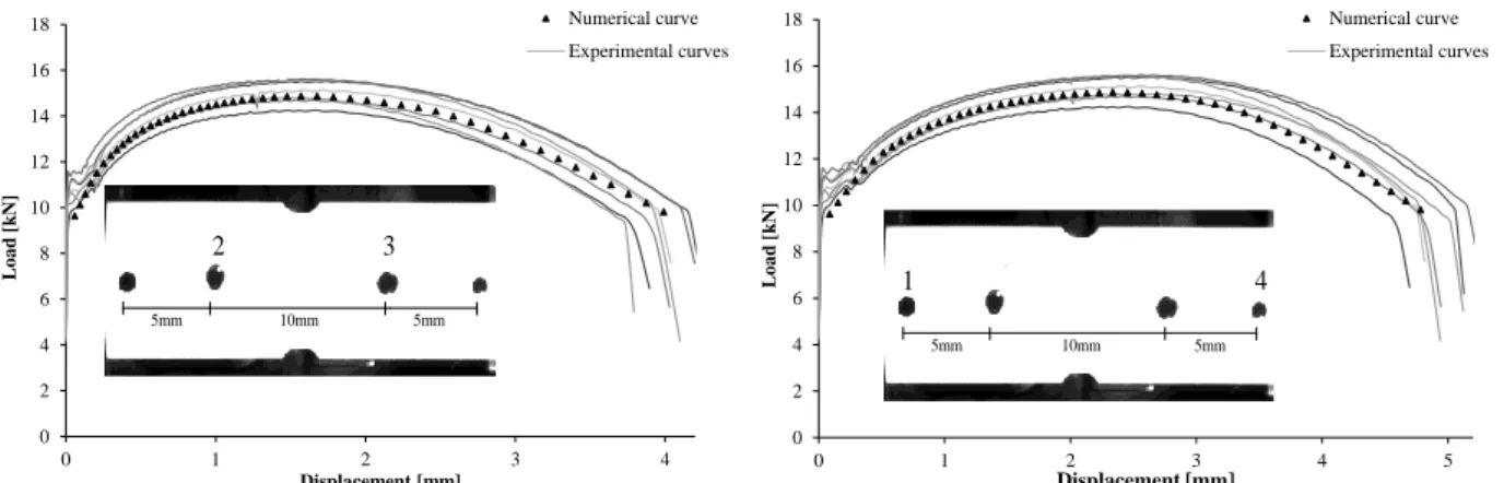
The same procedure was adopted for the notched cylindrical specimens in order to compute the experimental response. Due to notched influence, the specimens’ failure always occurred in region captured by the camera. The experimental load-displacements curves with numerical curve for the notched specimens are present in Figure 13 and 14. For both sets of specimens, CE and CES, the relative displacement was computed from two pairs of circular marks (1-4 and 2-3). A very good agreement between the numerical and experimental results, independently of the marks used.

0 2 4 6 8 10 12 14 0 0.5 1 1.5 2 2.5 L o a d [ k N] Displacement [mm] Numerical curve Experimental curves 1 2 3 4 10mm 5mm 5mm 0 2 4 6 8 10 12 14 0 0.5 1 1.5 2 2.5 3 L o a d [ k N] Displacement [mm] Numerical curve Experimental curves 1 2 3 4 10mm 5mm 5mm

Fig 13. Experimental load-displacements curves and numerical response of cylindrical specimens with small notch, CE: a) measured displacement between circular marks 2 and 3; b) measured displacement between

0 2 4 6 8 10 12 14 16 18 0 1 2 3 4 L o a d [ k N] Displacement [mm] Numerical curve Experimental curves 1 2 3 4 10mm 5mm 5mm 0 2 4 6 8 10 12 14 16 18 0 1 2 3 4 5 L o a d [ k N] Displacement [mm] Numerical curve Experimental curves 1 2 3 4 10mm 5mm 5mm

Fig 14. Experimental load-displacements curves and numerical response of cylindrical specimens with large notch, CES: a) measured displacement between circular marks 2 and 3; b) measured displacement between

circular marks 1 and 4.

The numerical simulations performed in ANSYS® 12.1 allowed computing the history of the parameters included in JC model for the critical region of the specimens. In addition to the tests described in this paper, test on Dog-bon and plate with circular hole specimens were also used in the derivation of the JC model parameters, as described by Pereira (2011) and Pereira et al. (2012). The equivalent plastic strain and stress triaxiality at fracture, for the specimens used in monotonic tensile tests, allowed the computation of the material constants, C₁0.85,

2 2.44

C  and C₃  4.67, by method of least squares. The ductility/damage curve for S185 structural steel is represented in Figure 15.

To obtain the KD model to monotonic fracture, the VGI_monotoniccritical was computed for all sets of specimens, considering the constant suggested by the authors, C₁1.5. In order to minimize the coefficient of variation of VGI_monotoniccritical for each set of specimens, an enhanced C₁0.72

constant was obtained. For this procedure the results obtained by Pereira et al. (2012) using plane specimens were also taking into account (Table 2).

0.0 0.4 0.8 1.2 1.6 2.0 0.0 0.2 0.4 0.6 0.8 1.0 1.2 εf Triaxiality CL CE CES LP PLF Johnson-Cook





Table 2. Critical monotonic void growth index: KD model and KD model modified Specimens ( 1 1.5) critical monotonic VGI C  ( 1 0.72) critical monotonic VGI C  CL 2.2 1.7 CES 4.6 2.0 CE 3.8 1.5 PFE 2.9 2.1 LP 1.9 1.4 Mean 3.11 1.77 σ 1.01 0.27 CoV [%] 32.48 15.28

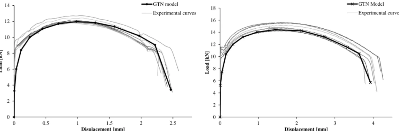
In relation to the calibration of the GTN model, numerical simulations of notched cylindrical specimens, CE and CES, were run explicit in ABAQUS® 6.1. The constants of GTN model were detemined using a fitting procedure between the numerical and experimental response. This plasticity model for monotonic fracture, allows to describe the monotonic behaviour of material included the loss of strength capacity at fracture, as we can see in the Figure 16, that represented the experimental and numerical load-displacement curves for CE and CES. The analysis of this figure confirms a good agreement between experimental and numerical results. The constants of GTN model for S185 structural steel are expressed in the Table 3.

The modelling of monotonic fracture in ABAQUS® involves the introduction of a new constant related with the finite element mesh size. Therefore, for different mesh sizes, also distinct constants are obtained. This effect has considerable influence, mainly in the constants that define the fracture instant, in particular, in the critical and failure porosity. As such, the finite element models should be evaluated using the same mesh density in order to minimize this effect in the numerical results. 0 2 4 6 8 10 12 14 0 0.5 1 1.5 2 2.5 L o a d [ k N] Displacement [mm] GTN model Experimental curves 0 2 4 6 8 10 12 14 16 18 0 1 2 3 4 L o a d [ k N] Displacement [mm] GTN Model Experimental curves

Figure 16. Experimental and numerical load-displacement curves: a) CE test series; b) CES test series.

Table 3. Constants of the GTN model

0 f 1E-05 fN 0.001 N  0.45 fC 0.11 N s 0.05 fF 0.08

CONCLUSIONS

A feature-tracking method was used in monotonic tensile tests performed in three series of cylindrical specimens. This image-based tracking method allowed to obtain the experimental load-displacement curves for the tests specimens with suitable accuracy.

The experimental response was used to calibrate the plasticity model with isotropic hardening involved in the finite element models. A very good correlation was found between the numerical and experimental results. Hence, the history of stress triaxiality and equivalent plastic strain for the critical region was computed successfully. These results were used to calibrate the JC and KD models for monotonic fracture. In particular, for the KD model a new constant, C1 0.72, which affects the stress triaxiality, was proposed to minimize the

coefficient of variation for the VGI_monotoniccritical computed in each series of tested specimens.

For the calibration of the GTN model, an explicit analysis was run in ABAQUS®. This analysis allowed to evaluate the influence of the mesh size in the finite element procedures. In fact, for different mesh sizes, distinct constants were obtained for the critical and failure porosity. Thus, the determination of the GTN parameters resulted in a compromise between the use of equal mesh density in the critical zones and the experimental results, and the correlation of both series of specimens. However, it was verified that the GTN model was able to describe satisfactorily the cylindrical notched specimens behaviour included the final degradation of the specimens.

REFERENCES

Coppola T, Cortese L, Folgarait P. The effect of stress invariants on ductile fracture limit in steels. Engineering Fracture Mechanics, 2009, 76: 1288–1302.

Gurson AL. Continuum theory of ductile rupture by void nucleation and growth. Part I: Yield criteria and flow rules for porous ductile media. Journal of Engineering Materials and Technology, 1977, 99(1): 2-15.

Johnson GR, Cook WH. Fracture characteristics of three metals subjected to various strains, strains rates, temperatures and pressures. Engineering Fractures Mechanics, 1985, 21(1):33-48.

Kanvinde AM, Deierlein GG. Cyclic void growth model to assess ductile fracture initiation in structural steels due to ultra-low cycle fatigue. Journal of Engineering Mechanics,2007, 133(6): 701-712.

Xavier J; Custódio P, Morais J, Guedes R. Assessing mechanical properties of a polymer material by a video extensometer technique. 7th EUROMECH Solid Mechanics Conference, J. Ambrosio et. al. (Eds.), 7-11 September, 2009, pp. 253-260, IST, Lisbon, Portugal.

ANSYS. Swanson Analysis Systems, Inc, Houston, Version 12.0, 2009.

ABAQUS. User’s manual version 6.10, Hibbitt, Karlsson, and Sorensen, Inc., Providence, R.I, 2010.

Wierzbicki T, Bao Y, Lee Y-W, Bai Y. Calibration and evaluation of seven fracture models. International Journal of Mechanical Sciences, 2005, 47:719–43.

Grédiac M. The use of full-field measurement methods in composite material characterization: Interest and limitations. Composites Part A: Applied Science and Manufacturing, 2004, 35(7-8):751-761

Sutton M, Orteu J-J, Schreier H. Image correlation for shape, motion and deformation measurements: basic concepts, theory and applications. Springer, 2009, ISBN#: 978-0- 387-78746-6.

13. Schmidt, T. Tyson, J. and Galanulis,

Pan B, Qian K, Xie H and Asundi A. Two-dimensional digital image correlation for in-plane displacement and strain measurement: a review Measurement Science Technology, 2009, 20 062001.

Rotinat R, bi Tié R, Valle V, Dupré J.-C. Three Optical Procedures for Local Large-Strain Measurement. Strain, 2001 37(3): 89–98.

Dahl KB, Malo KA. Planar Strain Measurements on Wood Specimens, Experimental Mechanics, 2009 49(4): 575-586.

Surrel Y. Design of algorithms for phase measurements by the use of phase stepping Applied Optics, 1996, 35(1): 51-60.

Avril S, Vautrin A, Surrel Y. Grid Method: Application to the Characterization of Cracks, Experimental Mechanics, 2004, 44(1): 37-43.

Franke S, Franke B, Rautenstrauch K. Strain analysis of wood components by close range photogrammetry. Materials and Structures, 2007 40(1): 37-46.

Pereira J. Behavior of steel components under the action of monotonic and cyclic extreme loading. University of Trás-os-Montes e Alto Douro, September 2011 (in Portuguese).

Pereira J, de Jesus A, Xavier J. Modelling monotonic behaviour in steel components supported by image-based methods. 15th International Conference on Experimental Mechanics, 2012, Porto, Portugal.