Statistical methods to study adaptability and stability in breeding lines of food-type soybeans

ABSTRACT: The grains of food-type soybean cultivars, which are characterized by the absence of lipoxygenases and the presence of

high levels of proteins and isoflavones, are regarded as functional

foods with high acceptance by consumers. However, few cultivars

of food-type soybeans are currently available in the Brazilian market.

The aim of this work was to study the adaptability and stability

of various genotypes of food-type soybeans and to compare the

performance of methods, which are based on analysis of variance,

non-parametric, regression, multivariate and mixed models. Ten

lines of food-type soybeans obtained from the Breeding Program

of Soybeans for Human Consumption of the State University of

Londrina (UEL/BPSHC) and two commercial varieties, the

food-type cultivar BRS 257 and the cultivar BMX Potência RR, were

evaluated in the counties of Londrina, Guarapuava, Ponta Grossa

PLANT BREEDING -

Article

Statistical methods to study adaptability and

stability in breeding lines of food-type soybeans

Nelson da Silva Fonseca Junior2_{, Wilmar Ferreira Lima}2_{, Cássio Egidio Cavenaghi Prete}1

1.Universidade Estadual de Londrina - Agronomia - Londrina (PR), Brazil. 2.Instituto Agronômico do Paraná - Melhoramento Vegetal - Londrina (PR), Brazil.

*Corresponding author: leandrosag@uel.br Received: Feb. 9, 2017 – Accepted: Aug. 14, 2017

and Pato Branco, Paraná, Brazil, during the two sowing seasons of

the harvest of 2014/2015. The characteristic evaluated was grain

yield. The adaptability parameters of Eberhart and Russel and

Cruz methods showed high correlations with the Wricke model.

The parameters provided by the analyses of Lins and Binns and

REML/BLUP showed higher grain yield associations and moderated

correlations with the Eskridge parameters. The AMMI offered the

possibility of use in conjunction with the other methodologies. When

yield, adaptability and stability were considered, the genotypes

UEL 110, UEL 122, UEL 121 and UEL 123 demonstrated potential

for the development of new cultivars of food-type soybeans in

which lipoxygenases are absent.

INTRODUCTION

The soybean (Glycine max (L.) Merrill) is recognized

by the U.S. Food and Drug Administration (FDA) as a

functional food. Containing approximately 40% protein with a balanced proportion of amino acids that are essential to the human diet, soy protein can reasonably replace protein from meat and dairy products (Day 2013). In addition, soybeans are rich in minerals, vitamins and isoflavones, and the latter are associated with the prevention or reduced incidence of several chronic degenerative diseases (Rimbach et al. 2008) and display oestrogenic and antioxidant activities (Liu et al. 2010).

Despite the clear benefits of soybeans and their derivatives consumption, less than 5% of the soybean crop produced is intended for human consumption (Hirakuri and Lazarotto 2014). This is in part due to its

unpleasant flavor, known as beany flavor, which results

from the action of lipoxygenase enzymes (LOXs) (Silva et al. 2012). Consequently, the genetic elimination of LOXs improves the sensory characteristics of soybean foods due to the lower production of hexanal compounds. Genotypes considered triple null (those that display a total absence of LOXs in grains) can be classified as food type and offer special features for human consumption (Silva et al. 2012).

According to the Ministério da Agricultura, Pecuária e Abastecimento (MAPA) data, only 15 food-type soybean cultivars have been recorded, whereas 1524 grain- type cultivars have been recorded (MAPA 2016). Therefore, the expansion of food-type soybean agribusiness depends on the development of breeding programmes that aim to develop genotypes with high agronomic value (Destro et al. 2013; Freiria et al. 2016).

For the commercial release of new cultivars, it is necessary to study various genotypes performances in different cultivation regions to control the interaction of plant genotype with the environment (GE). To minimize the effects of the GE interaction, it is necessary to analyze the adaptability and stability of each cultivar so as to identify genotypes with predictable behavior that are responsive to environmental variations under both specific and general conditions (Cruz et al. 2004).

Several methods to study the adaptability and stability of plant cultivars have been described. These methods are based on analysis of variance (Plaisted and Peterson 1959; Wricke

1965; Annicchiarico 1992) or on non-parametric (Lin and Binns 1988; Huenh 1990), regression (Finlay and Wilkinson 1963; Eberhart and Russell 1966; Tai 1971; Verma et al. 1978; Cruz et al. 1989; Storck and Vencovsky 1994), multivariate analysis (Zobel et al. 1988; Crossa 1990; Yan et al. 2000; Nascimento et al. 2013) or mixed models (Resende 2004).

The choice of method for assessing adaptability and stability is linked to the number of available environments as well as to the type of information and the level of experimental precision required (Cruz et al. 2004). With this in mind, several studies of soybean crops (Silva and Duarte 2006), beans (Pereira et al. 2009), corn (Scapim et al. 2010) and cotton (Silva Filho et al. 2008) have been conducted to identify the best methods of assessing these parameters, as well as their combinations, with the purpose of increasing the available precision for the selection and/ or indication of the best genotypes.

The aim of this work was to study the adaptability and stability of various genotypes of food-type soybeans and to compare the performance of methods, which are based on analysis of variance, non-parametric, regression, multivariate and mixed models.

MATERIAL AND METHODS

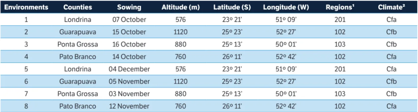
Twelve soybean genotypes, including 10 lines from the Breeding Program of Soybeans for Human Consumption of the State University of Londrina (UEL/BPSHC) and two commercial varieties (Table 1), were evaluated. The genotypes were sown in the counties of Londrina, Guarapuava, Ponta Grossa and Pato Branco, Paraná, Brazil, during the harvest of 2014/2015 in two seasons of sowing, totalling eight environments (Table 2).

The experimental plants were installed mechanically using a plot seeder in four lines (with five metres long spaced 0.45 m from each other, with 13 to 16 plants per metre) in a complete random block design with four replications. The

seeds were treated with Vitavax-Thiram® _{(carboxanilide}

and dimethyldithiocarbamate) at a concentration of 250 mL per 100 kg of seeds and inoculated at the time

of sowing with strains of Bradyhizobium japonicum and

B. elkanii at a concentration of 109 _{viable cells per mL. A}

no-tillage management system was used.

the typical colouring of mature pods (Fehr and Caviness 1977). The two outer lines of the plot, as well as plants within 0.5 m of each end of the centre line, were removed, yielding a useful area of 3.6 m². The evaluated

characteristic was grain yield (t.ha–1_{), corrected to 13%}

humidity.

Initially, an individual analysis of variance was performed. After verifying the magnitudes of the residual mean squares, a joint analysis of variance was performed. The effects of genotypes were considered fixed, and those related to the environment were considered random.

The analysis of adaptability and stability was performed using the methods of Wricke (1965), Eberhart and Russell (1966), Lin and Binns (1988), Cruz et al. (1989), Eskridge (1990), Zobel et al. (1988) and Resende (2007).

The statistical stability of the Wricke (1965) method, called

ecovalence (ϖ_i) was estimated according to the equation:

.

¹Edaphoclimatic regions, second Kaster and Farias (2012);²According to Köppen-Geifer. Table 1. Morphological and chemical properties of 12 evaluated soybean genotypes.

Lines/Cultivars Grow type Seed coat color

Hilum color

Weight of 100 grains*

Oil* (%)

Protein* (%)

Isoflavones¹*

(mg·100g-1₎ Lipoxygenases²

UEL 101 Indeterminate Yellow Black 13.36 19.85 40.88 131.36 Null

UEL 110 Determined Yellow Yellow 15.20 22.02 38.76 222.34 Null

UEL 112 Indeterminate Yellow Yellow 12.83 20.78 39.64 147.10 Null

UEL 113 Indeterminate Yellow Yellow 13.71 20.93 39.19 164.80 Null

UEL 114 Determined Yellow Brown 13.50 22.15 38.40 162.76 Null

UEL 115 Indeterminate Yellow Brown 13.26 22.49 38.75 168.89 Null

UEL 121 Indeterminate Yellow Brown 12.95 21.38 38.79 213.91 Null

UEL 122 Indeterminate Yellow Brown 12.92 21.11 39.78 214.04 Null

UEL 123 Indeterminate Yellow Brown 14.11 21.86 39.12 184.63 Null

UEL 153 Determined Yellow Brown 12.06 19.87 40.32 276.37 Null

BRS 257 Determined Yellow Brown 14.66 20.34 41.15 278.61 Null

BMX Potência Indeterminate Yellow Brown 12.06 --- --- --- Presence

.

¹Sum of chemical forms aglycones. 7-O-β-D-glycosides. 6 ‘-O- malonyl -7-O-β-D-glycosides and 6 “-O-acetyl-7-O-β-D-glycosides; ² Null: represents total absence of lipoxygenases enzymes in grains; and Presence: represents lipoxygenases enzymes in the presence; *Mean obtained in two seasons of seeding in the municipality of Londrina in 2013/2014.

Table 2. Location and climatic characterization of eight environments in the State of Paraná.

Environments Counties Sowing Altitude (m) Latitude (S) Longitude (W) Regions¹ Climate²

1 Londrina 07 October 576 23º 21’ 51º 09’ 201 Cfa

2 Guarapuava 15 October 1120 25º 23’ 52º 27’ 102 Cfb

3 Ponta Grossa 16 October 880 25º 13’ 50º 01’ 103 Cfb

4 Pato Branco 14 October 760 26º 11’ 52º 42’ 102 Cfa

5 Londrina 04 December 576 23º 21’ 51º 09’ 201 Cfa

6 Guarapuava 05 November 1120 25º 23’ 52º 27’ 102 Cfb

7 Ponta Grossa 03 November 880 25º 13’ 50º 01’ 103 Cfb

8 Pato Branco 12 November 760 26º 11’ 52º 42’ 102 Cfa

where Yij is the mean of the genotype i in environment j;

Yi is the mean of the genotype i in all environments; Yj

is the mean of the environment j for all genotypes; and 

Y.. is the overall mean. The cultivars with low ϖi values

are considered stable, which indicates that these cultivars have smaller deviations in relation to the environment.

The method of Lin and Binns (1988) is estimated by:

(1)

where P_iis the estimation of the stability parameter of

the cultivar i; X_ijis the grain yield of the ith cultivar in the

jth _{environment; M}

j is the maximum response observed

among all the cultivars in environment j; n is the number

of environments. The decomposition of this estimator

(P_i) was performed and divides in favorable (P_if) and

unfavorable (P_id) environments.

The mathematical models for the methods of Cruz et al. (1989) and Eberhart and Russell (1966) are similar. The difference is in the introduction of the regression coefficient in unfavorable environments proposed by the model of Cruz et al. (1989), forming two straight segments. The mathematical model in the bissegmented method of Cruz et al. (1989) is estimated by:

genotypes) in the environment j (j = 1, 2, ..., E environ-

ments); µ is the mean of the treatments; gi is the fixed effect

of genotype i; ajis the fixed effect of the environment j;

λk is the k

th _{singular value (scalar) of the original interaction}

matrix (denoted by GE); γik is the element corresponding

to the ith _{genotype, in the k}th _{singular vector of each}

column in the matrix GE; ajk is the element corresponding

to the jth _{environment in the k}th _{singular vector line of}

the matrix GE; ρij is the residue associated with the term

(gEij of the classical interaction of genotype i with the

environment j; εij is the experimental error.

In the REML/BLUP analysis (Resende 2007) was used the statistical model for genetic evaluation for higher values of the harmonic mean of the genotypic values:

where β₀i = general mean of genotype i (i = 1.2, ..., g);

β₁i = linear response of the genotype i to environmental

variation; I_j = environmental index (j = 1.2,...,);

δij = deviation of regression; εij = mean experimental error.

T(Ij) = 0, if Ij < 0 and equal to Ij + I + If Ij > 0, being I+

corresponds to the mean of the indexes Ij positive. The

model of Eberhart and Russell (1966) is explained by:

Yij = β10i + βiIj + δij +εj. The hypotheses ((H0: β1i = 1) and

(H₀: β₁i + β2i) = 1) were tested by the test tα, m, where α is

the level of significance, and m the degrees of freedom

of the residue.

The methodology proposed by Eskridge (1990) is based on the compounds estimation of safety first, as an adaptation of the model proposed by Kataoka (1963) for risks financial operations. The parameters were EV, FW, SH and ER, estimated with the inclusion of the following variance compounds: variance between environments (S ˆ2

xi ) in EV; the Finlay and Wilkinson linear regression

coefficient (βˆ₁i) in FW; the Shukla variance (σˆi) in SH;

and the Finlay and Wilkinson linear regression coefficient

(βˆ₁i) plus the deviations variance of the Eberhart and

Russel linear regression (δˆji) in ER.

For the use of the method AMMI (Zobel et al. 1988), the model applied was:

(3) (5)

(4)

where Yij is the mean response of genotype i (i = 1, 2, ..., G

where Y is the vector of observations (phenotypic values),

r is the vector of the local-repetition combinations effects

added to the general mean, g is the vector of the genotypic

effects, i is the vector of the interaction genotypes vs.

environments effects, being e the error vector. The

uppercase letters represent the incidence matrices for these effects.

In the REML/BLUP analysis, the selection by the highest values of the harmonic mean of the genotypic values (MHVG) has a simultaneous effect in the selection for grain yield and stability. The adaptability refers to the relative performance of the genotypic values (PRVG) according to the environment. The simultaneous selection for yield, stability and adaptability can be performed by the method of the harmonic mean of the relative performance of the genetic values (MHPRVG).

Spearman’s correlation coefficient was used to verify similarities and differences between the parameters of adaptability and stability estimates obtained using different methods, and the significance of the differences was verified by Student’s t-test. For the AMMI analysis was considered the weighted average of the absolute scores (MPEA) of the first two principal components for each genotype, weighted by the percentage of variance explained by each component.

RESULTS AND DISCUSSION

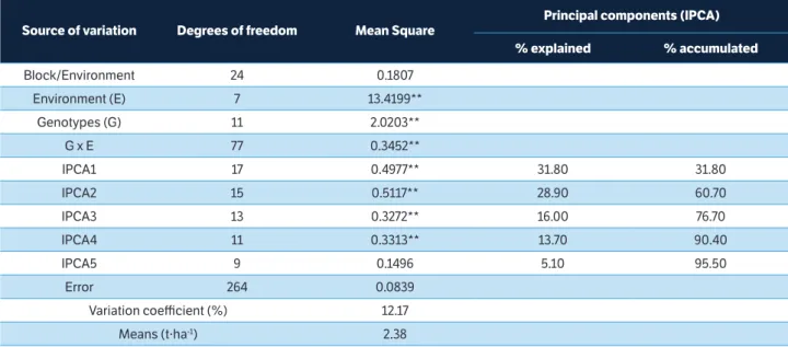
The joint analysis of variance indicated that the sources of variation (genotype - G, environment - E, and the interaction GE) were significant (p ≤ 0.01). This allowed us to infer that the environments evaluated were distinct and the genotypes presented differentiated performance in response to environmental variations

(Table 3). The general mean grain yield was 2.38 t.ha–1_;

in the environments tested, the value of this parameter

ranged from 1.51 to 3.05 t.ha–1_. 

In the AMMI analysis, the first principal axis (IPCA 1) accounted for 31.80% of the pattern associated with the GE interaction. In addition to the IPCA 2, the accumulated was 60.70%. When the contribution of the other axes was considered, significance (p < 0.01) was observed in the IPCA 3 and IPCA 4.

Maia et al. (2006) and Yokomizo et al. (2013) analysed the adaptability and stability of soybean genotypes and found that the values of the first two axes explained the range of

53 to 58 % of the variance in SS_GE. According to Oliveira

et al. (2003) and Gauch Jr. (2013), as the number of axes selected increases, the percentage of “noise” also increases, reducing the predictive power of the AMMI analysis, i.e., the excessive inclusion of multiplicative terms can reduce the accuracy of the analysis. Therefore, only the IPCA 1 and IPCA 2 axes were considered in the AMMI analysis.

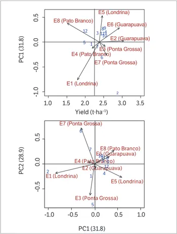
The genotypes or environments with points near the origin of the coordinate system of the biplot graphic are considered more stable (Duarte and Vencovsky 1999). The

AMMI biplot 1 (mean of grain yield vs. IPCA 1) (Figure 1)

showed that the most stable genotypes were BRS 257, UEL 114, UEL 101, UEL 122 and UEL 123. Among these, the most prominent lines were UEL 122 and UEL 123, both of which showed yields above the overall average. Thus, these lines demonstrated general adaptability in both sowing seasons, but with higher responses when sown in the county of Guarapuava.

The use of an AMMI biplot 2 (IPCA 1 vs. IPCA 2)

(Figure 1) permits correction for possible distortions in the analysis or interpretation produced using a single dimension (Yokomizo et al. 2013). In general, the genotypic behavior presented confirmed the previous analysis and indicated that the genotypes of lines UEL 110, UEL 153, UEL 115 and UEL 121 are stable. The cultivar BMX Potência RR and the lines UEL 112 and UEL 113 were classified as being of low stability and specifically adapted to the counties of Londrina and Ponta Grossa in the first sowing season and to the county of Ponta Grossa in the second season.

By analyzing the environments, the counties of Ponta Grossa and Londrina were found to be the main contributors to the GE interaction in both sowing seasons, with higher environmental scores in the interaction axis when the

Source of variation Degrees of freedom Mean Square

Principal components (IPCA)

% explained % accumulated

Block/Environment 24 0.1807

Environment (E) 7 13.4199**

Genotypes (G) 11 2.0203**

G x E 77 0.3452**

IPCA1 17 0.4977** 31.80 31.80

IPCA2 15 0.5117** 28.90 60.70

IPCA3 13 0.3272** 16.00 76.70

IPCA4 11 0.3313** 13.70 90.40

IPCA5 9 0.1496 5.10 95.50

Error 264 0.0839

Variation coefficient (%) 12.17

Means (t·ha-1_{) 2.38}

Table 3. Analysis of variance for grain yield of 12 genotypes of soybean food type, including the participation of the interaction genotype

vs. environment (GE) according to the main additive effect and multiplicative interaction (AMMI) in eight environments in the Paraná State.

AMMI 2 was considered. According to Oliveira et al. (2003), environmental stability contributes to the reliability of genotype ordering in test environments in relation to the classification for the average of the tested environments. Our results did not correspond to those obtained using the environmental indices proposed by Cruz et al. (1989) and Lin and Binns (1988). In those indices, the counties considered unfavorable were Pato Branco (both sowing seasons) and Londrina (first sowing season).

The environmental index is a measure of environmental quality that allows classification of favorable or unfavorable environments. However, in the case of grain yield, the strongest criticism to the use of this criterion relates to the association of the environmental index (independent variable in the regression) with the dependent variable (Maia et al. 2006).

It was verified by the Wricke methodology (Table 4) that the UEL 153, UEL 114, UEL 101, UEL 121 and UEL 110 lines, which are considered the most stable lines, displayed the lowest ecovalence (ϖi) values. However, the genotypes BMX Potência RR, UEL 112 and UEL 113 were the most unstable in the face of environmental changes, and these results were concordant with the results of the AMMI analysis.

In the methodology proposed by Eberhart and Russell (1966), it was observed that the UEL 101 line and the BRS

1.0 1.5 2.0 2.5 3.0 3.5

-1.0

-0.5

0.0

0.5

Yield (t·ha–1₎

PC1 (31.8)

E1 (Londrina)

E2 (Guarapuava)

E3 (Ponta Grossa) E4 (Pato Branco)

E5 (Londrina)

E6 (Guarapuava)

E7 (Ponta Grossa) E8 (Pato Branco)

1

2

3 4

5

6 7

89 10 11 12

-1.0 -0.5 0.0 0.5 1.0

-0.5

0.0

0.5

PC1 (31.8)

PC2 (28.9)

E1 (Londrina)

E2 (Guarapuava)

E3 (Ponta Grossa) E4 (Pato Branco)

E5 (Londrina) E6 (Guarapuava)

E7 (Ponta Grossa)

E8 (Pato Branco)

1 2

3

4

5 6

7

8 9 10₁₁

12

Figure 1. Biplot AMMI to yield of grain data of food type soybeans, with 12 soybean genotypes (1: BRS 257; 2: Potência; 3: UEL 101; 4: UEL 110; 5: UEL 112; 6: UEL 113; 7: UEL 114; 8: UEL 115; 9: UEL 121; 10: UEL: 122; 11: UEL 123; 12: UEL 153) and eight environments in the Paraná State, 2014/2015.

Genotypes Grain Yield (t·ha-1₎

Ecovalence (ϖi)

Lin & Binns

(1988) Eberhart and Russel Cruz, Torres and Vencovsky

Pi Pif Pid β1i δ²di R² (%) β1i β1i + β2i δ²di R² (%)

UEL 101 2.324 1.00 0.35 0.28 0.51 0.7529* 0.0008NS _{89.46 0.7230* 0.9416}NS _0.0958NS _90.35

UEL 110 2.539 1.31 0.21 0.08 0.35 1.0236NS _{0.0338* 86.19 1.0922}NS _0.5903NS _{0.2163* 88.63}

UEL 112 1.970 4.65 0.70 0.62 1.00 1.1506NS _{0.1654** 69.85 1.1688}NS _1.0358NS _{0.8914** 69.96}

UEL 113 2.441 3.25 0.27 0.22 0.46 0.9684NS _{0.1142** 69.35 0.9326}NS _1.1947NS _{0.6362** 69.96}

UEL 114 2.321 0.98 0.33 0.25 0.51 1.0042NS _0.0200NS _{88.91 1.0159}NS _0.9302NS _{0.1956* 88.99}

UEL 115 2.469 1.96 0.29 0.23 0.47 0.8165NS _{0.0496** 75.50 0.8381}NS _0.68022NS _{0.3340** 75.84}

UEL 121 2.497 1.20 0.24 0.13 0.40 1.1355NS _0.023NS _{90.54 1.1511}NS _1.0371NS _{0.2085* 90.65}

UEL 122 2.517 2.49 0.27 0.17 0.43 1.3591** 0.0406** 90.73 1.2268* 2.1949** 0.1224NS _96.16

UEL 123 2.458 1.32 0.24 0.08 0.36 0.9871NS _{0.0339* 85.26 0.9924}NS _0.9537NS _{0.2634* 85.28}

UEL 153 1.991 0.69 0.65 0.44 0.84 1.1974NS _-0.0048NS _{96.65 1.1805}NS _1.3048NS _0.0750NS _96.77

BRS 257 2.159 1.33 0.45 0.39 0.56 0.7947* 0.0207NS _{83.18 0.9154}NS _{0.0323** 0.0558}NS _95.30

Potência 2.874 6.38 0.03 0.04 0.01 0.8099NS _{0.2333** 45.70 0.7633* 1.1045}NS _{1.1989** 46.65}

Table 4. Estimates of the parameters of adaptability and phenotypic stability, obtained by methods of Wricke (1965) (Ecovalence-ϖ_i), Lin and Binns (1988), Eberhart and Russell (1966) and Cruz et al. (1989), for the character of grain yield in 12 soybean genotypes in eight environments in the State of Paraná, 2014/2015.

NS _{, * and **: no significant, significant at the level of 5 and 1%, respectively, by the test t (H}

257 cultivar presented values of β_1i < 1; these varieties are therefore considered adapted to unfavorable environments,

whereas the UEL 122 line, with β_1i > 1, was considered

to be adapted only to favorable environments. The other genotypes were considered to be of wide adaptability. The

genotypes considered stable (δ ²_di = 0) were UEL 101, UEL

114, UEL 121, UEL 153 and BRS 257 (Table 4).

The parameters of adaptability and stability of Eberhart and Russell (1966) are similar to those used by Cruz et al. (1989). However, the method of Cruz et al. (1989), which considers two regression lines (one for unfavorable environments and other for favorable environments), permitted better conclusions about the behavior of genotypes with respect to front environmental variations. This method considers the ideal genotype one that is

less responsive to unfavorable environments (β₁ < 1.0),

responsive to favorable environments (β₁ + β₂ > 1.0), has

high stability (δ_ij = 0) and has good grain yield. In the

studied materials, such a genotype was not identified (Table 4).

The cultivar BMX Potência RR and the line UEL 101 were less responsive in unfavorable environments (β1i < 1.0); the remaining genotypes, with the exception of UEL 122, showed average responsiveness in unfavorable environments (β1i = 1.0). The UEL 122 line was highly responsive in favorable environments (β1i + β2i > 1.0); the remaining genotypes, with the exception of the cultivar BRS 257, displayed wide adaptability to favorable environments (β1i + β2i = 1.0). In relation to the stability parameter (δ² di), the genotypes that showed regression deviations close to zero and were therefore considered stable were the lines UEL 101, UEL 122 and UEL 153 and the cultivar BRS 257 (Table 4).

Low values of the coefficient of determination (R²) indicate high dispersion of the data and therefore low reliability in the type of environmental response determined by the regression analysis. However, the relevance of the stability parameter can be minimized under conditions in which the value of R² is greater than 80% (Cruz and Carneiro 2003). These conditions were found in the genotypes that presented stability by the methods of Eberhart and Russell (1966) and Cruz et al. (1989).

Unlike the results obtained using the methodologies of Wricke (1965), Eberhart and Russell (1966) and Cruz et al. (1989), the cultivar BMX Potência RR was the genotype

with the greatest adaptability and stability when the P_i

values obtained by the methodology of Lin and Binns (1988) were considered. This result can be explained by the

way in which the P_i statistics are estimated. The method

results in cultivars whose grain yields in each environment are close to the maximum, being considered as having greater adaptability and stability (Cruz and Carneiro

2003). In cases involving favorable (P_if) and unfavorable

(P_id) environments, the lowest values were attributed to

the genotypes BMX Potência RR, UEL 110, UEL 121 and UEL 123. This indicates that these genotypes show responsiveness to improvement in the environmental conditions and low yield losses in unfavorable environments (Table 4).

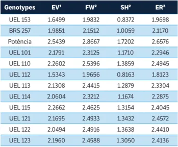
In the methodology proposed by Eskridge (1990), the genotypes with higher stability for grain yield were the cultivar BMX Potência RR and the lines UEL 110, UEL 115, UEL 121, UEL 122 and UEL 123, also with the highest values for the parameters EV, FW, SH and ER. Higher estimative from the FW and SH parameters represent a close genotype response to the average of the genotypic group response and higher values of ER indicated high predictability of the genotypes (Table 5).

The REML/BLUP model (Resende 2007) obtained results similar to those founded by the of Lin and Binns (1988) and Eskridge (1990) methods. In this analysis, the cultivar BMX

Table 5. Estimates of the stability parameters obtained by method of Eskridge (1990) for grain yield in 12 soybean genotypes in eight environments in the State of Paraná, 2014/2015.

Genotypes EV¹ FW² SH² ER²

UEL 153 1.6499 1.9832 0.8372 1.9698

BRS 257 1.9851 2.1512 1.0059 2.1170

Potência 2.5439 2.8667 1.7202 2.6576

UEL 101 2.1791 2.3125 1.1710 2.2946

UEL 110 2.2602 2.5396 1.3859 2.4945

UEL 112 1.5343 1.9656 0.8163 1.8123

UEL 113 2.1308 2.4415 1.2879 2.3304

UEL 114 2.0604 2.3212 1.1674 2.2875

UEL 115 2.2662 2.4625 1.3154 2.4045

UEL 121 2.1695 2.4933 1.3432 2.4572

UEL 122 2.0494 2.4916 1.3638 2.4410

UEL 123 2.1960 2.4588 1.3050 2.4136

¹EV: Safety-first index with variance across environments as stability parameter; ²FW: Safety-first index with Finlay and Wilkinson regression coefficient as stability parameter; ³SH: Safety-first index with Shukla variance as stability parameter; 4_{ER: Safety-first index with Finlay and Wilkinson regression}

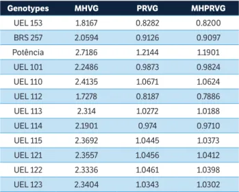
Genotypes MHVG PRVG MHPRVG

UEL 153 1.8167 0.8282 0.8200

BRS 257 2.0594 0.9126 0.9097

Potência 2.7186 1.2144 1.1901

UEL 101 2.2486 0.9873 0.9824

UEL 110 2.4135 1.0671 1.0624

UEL 112 1.7278 0.8187 0.7886

UEL 113 2.314 1.0272 1.0188

UEL 114 2.1901 0.974 0.9710

UEL 115 2.3692 1.0445 1.0373

UEL 121 2.3557 1.0456 1.0412

UEL 122 2.3336 1.0461 1.0398

UEL 123 2.3404 1.0343 1.0302

Potência RR presented the highest values for MHVG, PRVG and MHPRVG (Table 6). According to Borges et al. (2010), the MHVG values represent the actual amount of grain yield penalized by the instability, which facilitates the selection of the most productive and more stable lines. The MHPRVG values allow simultaneous selection for grain yield, stability and adaptability. In this case, the highest values were observed for the genotypes BMX Potência RR, UEL 110, UEL 121, UEL 122 and UEL 115 (Table 6).

Table 6. Stability of genotypic values (MHVG), adaptability of genotypic values (PRVG), stability and adaptability of genotypic values (MHPRVG) and for grain yield in 12 soybean genotypes in eight environments in the State of Paraná, 2014/2015.

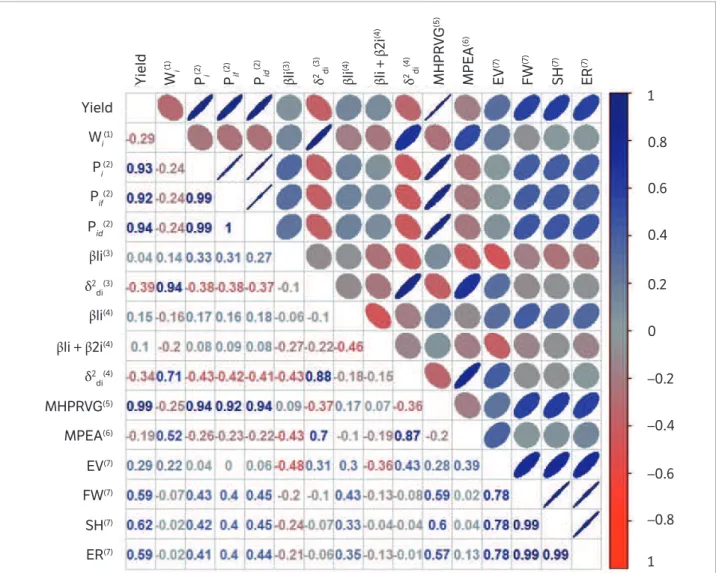
The possibility of using one or more parameters of stability obtained by different methods for the response prediction of a particular genotype to environmental changes requires the establishment of the level of association between these estimates (Franceschi et al. 2010). Depending on the degree of association, this can be an auxiliary measure in the choice of the stability parameter that results in the best adjustment and provides more essential information to base the concept of stability (Duarte and Zimmermann 1995).

In this work, high positive correlations were found between the ecovalence parameter of Wricke (1965) and the regression deviation of the models of Eberhart and Russell (1966) and Cruz et al. (1989). This result corroborates the results obtained by Cargnelutti Filho et al. (2007) and Paula et al. (2014). According to Pereira et al. (2009), high correlation indicates redundancy in the information provided. Therefore, the regression models recommended by Eberhart and Russell (1966) and/or Cruz et al. (1989) are able to measure the adaptability and stability

information provided by the Wricke model with reasonable accuracy and can replace it, as indicated by Silva and Duarte (2006).

The adaptability parameters of the Eberhart and Russell (1966) and Cruz et al. (1989) methods yielded non-significant correlations and can thus be viewed as complementary, emphasizing the importance of the fractionation of regression in favorable and unfavorable environments. For the stability parameter, a positive correlation of 0.88 between the two models was found, since for both the stability is measured by the regression deviations.

High positive correlations were found among the parameters provided by the Lin and Binns method (1988) and MHPRVG of the REML/BLUP (Resende 2007), a fact that seems to be associated with high participation of grain yield in the substantiation of both models (Figure 2). The methods based on analysis of variance (Wricke 1965), linear regression (Eberhart and Russell 1966) and AMMI (Zobel et al. 1988) presented no correlation with grain yield. Therefore, according to Cruz and Carneiro (2003), in these models special attention should be given to grain yield in addition to adaptability and stability.

The decomposition of the values of P_iin favorable

environments (P_if) and unfavorable environments (P_id) is

adopted in several works (Barros et al. 2008). However, there

was a high correlation with Pi, demonstrating redundancy

of the information transmitted.

Based on the methods of Wricke (1965), Eberhart and Russell (1966) and Cruz et al. (1989), the genotypes UEL 114, UEL 121 and UEL 153 were indicated as being of wide adaptability and stable. On the other hand, in the analysis of Lin and Binns (1988), Eskridge (1990) and REML/BLUP (Resende 2007), the genotypes classified as stable and adaptable were the cultivar BMX Potência RR and the lines UEL 110, UEL 121, UEL 122 and UEL 123. In the AMMI analysis, most of the genotypes, with the exception of UEL 113, UEL 112 and BMX Potência RR, possessed wide stability. Considering grain yield together with adaptability and stability, the genotypes UEL 110, UEL 122, UEL 121 and UEL 123 appear to offer potential for the development of new cultivars of food-type soybean varieties in which lipoxygenases are absent.

ORCID ID

G. H. Freiria

https://orcid.org/0000-0003-2786-3810

L. S. A. Gonçalves

https://orcid.org/0000-0001-9700-9375

F. F. Furlan

https://orcid.org/0000-0002-4441-2985

N. S. Fonseca Júnior:

https://orcid.org/0000-0003-2581-6017

W. F. Lima

https://orcid.org/0000-0003-4888-4282

C. E. C. Prete

https://orcid.org/0000-0003-0337-6874 Figure 2. Spearman correlation for the adaptability and stability parameters of each pair of methods and grain yield (t.ha-1_). 

1

0.8

0.6

0.4

0.2

0

–0.2

–0.4

–0.6

–0.8

1 Yield

W_i(1)

P

i

(2)

P_if(2)

P_id(2)

βli(3)

δ2 di

(3)

βli(4)

βli + _β2i(4)

δ2 di

(4)

MHPRVG(5)

MPEA(6)

EV(7)

FW(7)

SH(7)

ER(7)

Yield W

i

(1

)

Pi

(2)

Pif

(2)

Pid

(2)

β

li

(3

)

δ

2 di

(3

)

β

li

(4

)

β

li +

β

2i

(4

)

δ

2 di

(4

)

MHPR

V

G

(5)

MPEA

(6)

EV

(7

)

FW

(7

)

SH

(7

)

ER

(7

)

Parameters obtained by method of (1) _{Wricke (1965),} (2) _{Lin and Binns (1988) with decomposition in favorable and unfavorable environments,} (3) _{Eberhart and}

Russell (1966), (4) _{Cruz et al. (1989),} (5) _{REML/BLUP (Resende 2007),} (6) _{weighted mean of the absolute scores from PC1 and PC2 of AMMI (Zobel et al. 1988),}

Annicchiarico, P. (1992). Cultivar adaptation and recommendation

from alfalfa trials in northern Italy. Journal of Genetics and Plant Breeding, 46, 269-278.

Barros, H. B., Sediyama, T., Teixeira, R. C. and Cruz, C. D. (2008).

Análise paramétricas e não-paramétricas para determinação da

adaptabilidade e estabilidade de genótipos de soja. Scientia Agrária, 9, 299-309. http://dx.doi.org/10.5380/rsa.v9i3.11566.

Borges, V., Soares, A. A., Reis, M. S., Resende, M. D. V., Cornélio, V.

M. O., Leite, N. A. and Vieira, A. R. (2010). Desempenho genotípico

de linhagens de arroz de terras altas utilizando metodologia de

modelos mistos. Bragantia, 69, 833-841. http://dx.doi.org/10.1590/ S0006-87052010000400008.

Cargnelutti Filho, A., Perecin, D., Malheiros, E. B. and Guadagnin,

J. P. (2007). Comparação de métodos de adaptabilidade e

estabilidade relacionados à produtividade de grãos de cultivares de milho. Bragantia, 66, 571-578. http://dx.doi.org/10.1590/

S0006-87052007000400006.

Crossa, J. (1990). Statistical analysis of multilocations trials.

Advances in Agronomy, 44, 55-85. https://doi.org/10.1016/

S0065-2113(08)60818-4.

Cruz, C. D. and Carneiro, P. C. S. (2003). Modelos biométricos

aplicados ao melhoramento genético. 2. ed. Viçosa: UFV.

Cruz, C. D., Torres, R. A. and Vencovsky, R. (1989). An alternative

approach to the stability analysis proposed by Silva and Barreto.

Revista Brasileira de Genética, 12, 567-580.

Cruz, C. D., Regazzi, A. J. and Carneiro, P. C. S. (2004). Modelos

biométricos aplicados ao melhoramento genético. Viçosa: Editora

da UFV.

Cruz, C. D. (2016). Genes Software – extended and integrated with the R, Matlab and Selegen. Acta Scientiarum. Agronomy, 38,

547-552. http://dx.doi.org/10.4025/actasciagron.v38i3.32629.

Day, L. (2013). Proteins from land plants – Potential resources for

human nutritions and food security. Trends in Food Science &

Technology, 32, 25-42. http://dx.doi.org/10.1016/j.tifs.2013.05.005.

Destro, D., Faria, A. P., Destro, T. M., Faria, R. T., Gonçalves, L. S. A.

and Lima, W. F. (2013). Food type soybean cooking time: a review.

Crop Breeding and Applied Biotechnology, 13, 194-199. http://

dx.doi.org/10.1590/S1984-70332013000300007.

REFERENCES

Duarte, J. B. and Zimmermann, M. J. O. (1995). Correlation among yield

stability parameters in common bean. Crop Science, 35, 905-912.

http://dx.doi.org/10.2135/cropsci1995.0011183X003500030046x.

Duarte, J. B. and Vencovsky, R. (1999). Interação genótipos x

ambientes: uma introdução à analise AMMI. Ribeirão Preto:

Sociedade Brasileira de Genética.

Eberhart, S. A. and Russel, W. A. (1966). Stability parameters

for comparing varieties. Crop Science,6, 36-40. http://dx.doi.

org/10.2135/cropsci1966.0011183X000600010011x.

Eskridge, K. M. (1990). Selection of stable cultivars using a

safety-first rule. Crop Science, 30, 369-374. http://dx.doi.org/10.2135/

cropsci1990.0011183X003000020025x.

Fehr, W. R. and Caviness, C. E. (1997). Stages of soybean development.

Ames: Iowa State University of Science and Technology.

Finlay, K. W. and Wilkinson, G. N. (1963). The analysis of adaptation

in a plant breeding programme. Australian Journal of Agricultural

Research, 14, 742-754. http://dx.doi.org/10.1071/AR9630742.

Franceschi, L., Benin, G., Marchioro, V. S., Martin, T. N., Silva, R. R.

and Silva, C. L. (2010). Métodos para análise de adaptabilidade e

estabilidade em cultivares de trigo no estado do paraná. Bragantia,

69, 797-805. http://dx.doi.org/10.1590/S0006-87052010000400004.

Freiria, G, H., Lima, W. F., Leite, R. S., Mandarino, J. M. G., Silva, J. B.

and Prete, C. E. C. (2016). Productivity and chemical composition

of food-type soybeans sown on diferente dates. Acta Scientiarum.

Agronomy, 38, 371-377. http://dx.doi.org/10.4025/actasciagron.

v38i3.28632.

Gauch Jr., H. G. (2013). Simple protocol for AMMI analysis of yield

trials. Crop Science, 53, 1860-1869. http://dx.doi.org/10.2135/

cropsci2013.04.0241.

Hirakuri, M. H. and Lazzarotto, J. J. (2014). O agronegócio da soja

nos contextos mundial e brasileiro. Londrina: Embrapa Soja.

Huehn, M. (1990). Nonparametric measures of phenotypic stability.

Part 1: Theory. Euphytica, 47, 189-194. http://dx.doi.org/10.1007/

BF00024241.

Kaster, M. and Farias, J. R. B. (2012). Regionalização dos testes

de Valor de Cultivo e Uso e da indicação de cultivares de soja:

Kataoka, S. A. (1963). A Stochastic programming model. Econometrica, 31, 181-196. http://dx.doi.org/10.2307/1910956.

Kvitschal, M. V., Vidigal Filho, O. S., Scapim, C. A., Gonçalves-Vidigal, M. C., Sagrilo, E., Pequeno, M. G. and Rimoldi, F. (2009). Comparison of methods for phenotypic stability analysis of cassava (Manihot esculenta Crantz) genotypes for yield and storage root dry matter content. Brazilian Archives of Biology and Technology, 52, 163-175. http://dx.doi.org/10.1590/S1516-89132009000100022.

Lin, C. S. and Binns, M. R. (1988). A superiority measure of cultivar performance for cultivar x location data. Canadian Journal of Plant Science,68, 193-198. http://dx.doi.org/10.4141/cjps88-018.

Liu, Z., Kanjo, Y. and Mizutani, S. (2010). A review of phytoestrogens: Their occurrence and fate in the environment. Water Research, 44, 567-577. http://dx.doi.org/10.1016/j.watres.2009.03.025.

Maia, M. C. C., Vello, N. A., Rocha, M. M., Pinheiro, J. B. and Silva Júnior, N. F. (2006). Adaptabilidade e estabilidade de linhagens experimentais de soja selecionadas para caracteres agronômicos através de método uni-multivariado. Bragantia, 65, 215-226. http:// dx.doi.org/10.1590/S0006-87052006000200004.

MAPA. (2016). Ministério da Agricultura Pecuária e Abastecimento. Available at: http://extranet.agricultura.gov.br/php/proton/ cultivarweb/cultivares_registradas.php. Accessed on January 30, 2018.

Nascimento, M., Peternelli, L. A., Cruz, C. D., Nascimento, A. C. C., Ferreira, R. P., Bhering, L. L. and Salgado, C. C. (2013). Artificial

neural networks for adaptability and stability evaluation in alfalfa genotypes. Crop Breeding and Applied Biotechnology,13, 152-156.

http://dx.doi.org/10.1590/S1984-70332013000200008.

Oliveira, A. B., Duarte, J. B. and Pinheiro, J. B. (2003). Emprego da análise AMMI na avaliação da estabilidade produtiva em soja. Pesquisa Agropecuária Brasileira, 38, 357-364. http://dx.doi. org/10.1590/S0100-204X2003000300004.

Paula, T. O. M., Marinho, C. D., Souza, V., Barbosa, M. H., Peternelli, L. A., Kimbeng, C. A. and Zhou, M. M. (2014). Relationships between methods of variety adaptability and stability in sugarcane. Genetics Molecular Research,13, 4216-4225. http://dx.doi.org/10.4238/2014. June.9.7.

Pereira, H. S., Melo, L. C., Peloso, M. J. D., Faria, L. C., Costa, J. G. C., Díaz, J. L. C., Rava, C. A. and Wendland, A. (2009). Comparação de

métodos de análise de adaptabilidade e estabilidade fenotípica em feijoeiro-comum. Pesquisa Agropecuária Brasileira, 44, 374-383. http://dx.doi.org/10.1590/S0100-204X2009000400007.

Plaisted, R. L. and Peterson, L. C. (1959). A technique for evaluating the ability of selection the yield consistently in different locations or seasons. American Potato Journal, 36, 381-385. http://dx.doi.

org/10.1007/BF02852735.

R Development Core Team. (2012). R: a language and environment

for statistical computing. Vienna: R Foundation for Statistical Computing.

Resende, M. D. V. (2004). Métodos estatísticos ótimos na análise de experimentos de campo. Colombo: Embrapa Florestas.

Resende, M. D. V. (2016). Software Selegen-REML/BLUP: a useful tool for plant breeding. Crop Breeding and Applied Biotechnology, 16, 330-339.http://dx.doi.org/10.1590/1984-70332016v16n4a49.

Rimbach, G., Boesch-Saadatmandi, C., Frank, J., Fuchs, D., Wenzel, U.,

Daniel, H., Hall, W.I. and Weinberg, P. D. (2008). Dietary isoflavones in the prevention of cardiovascular disease – A molecular perspective. Food Chemical Toxicology, 46, 1308-1319. http://dx.doi.org/10.1016/j. fct.2007.06.029.

Scapim, A., Pacheco, C. A. P, Amaral Júnior, A. T., Vieira, R. A., Pinto,

R. J. B. and Conrado, T. V. (2010). Correlations between the stability and adaptability statistics of popcorn cultivars. Euphytica, 174, 209-218. http://dx.doi.org/10.1007/s10681-010-0118-y.

Silva, W. C. J. and Duarte, J. B. (2006). Métodos estatísticos para estudo de adaptabilidade e estabilidade fenotípica em

soja. Pesquisa Agropecuária Brasileira, 41, 23-30. http://dx.doi. org/10.1590/S0100-204X2006000100004.

Silva Filho, J. L., Morello, C. L., Farias, F. J., Lamas, F. M., Pedrosa, M. B. and Ribeiro, J. L. (2008). Comparação de métodos para avaliar a adaptabilidade e estabilidade produtiva em algodoeiro. Pesquisa Agropecuária Brasileira,43, 349-355. http://dx.doi.org/10.1590/

S0100-204X2008000300009.

Silva, J., Prudêncio, S., Carrão-Panizzi, M., Gregorut, C., Fonseca, F. and Mattoso, L. (2012). Study on the flavour of soybean cultivars by sensory analysis and electronic tongue. International Journal of Food Science Technology, 47, 1630-1638. http://dx.doi.

org/10.1111/j.1365-2621.2012.03013.x.

Storck, L. and Vencovsky, R. (1994). Stability analysis based on a bi-segmented discontinuous model with measurement errors in the variables. Revista Brasileira de Genética,17, 75-81.

Tai, G. C. C. (1971). Genotypic stability analysis and its application to potato regional trials. Crop Science,11, 184-190. http://dx.doi.

Verma, M. M., Chahal, G. S. and Murty, B. R. (1978). Limitations

of conventional regression analysis a proposed modification.

Theoretical and Applied Genetics,53, 89-91. http://dx.doi.

org/10.1007/BF00817837.

Vidigal Filho, P. S., Pequeno, M. G., Kvitschal, M. V., Rimoldi, F.,

Gonçalves-Vidigal, M. C. and Zuin, G. C. (2007). Estabilidade

produtividade de cultivares de mandioca-de-mesa coletadas no

Estado do Paraná. Semina: Ciências Agrárias, 28, 551-562. http://

dx.doi.org/10.5433/1679-0359.2007v28n4p551.

Wricke, G. (1965). Zur berechnung der ökovalenz bei sommerweizen

und hafer. Zeitschrift für Pflanzenzüchtung, 52, 127-138.

Yan, W., Hunt, L. A., Sheng, Q. L. and Szlavnics, Z. (2000). Cultivar evaluation and mega-environment investigation based on the GGE Biplot. Crop Science, 40, 597-605. http://dx.doi.org/10.2135/ cropsci2000.403597x.

Yokomizo, G. K., Duarte, J. B., Vello, N. A. and Unfried, J. R. (2013). Análise AMMI da produtividade de grãos em linhagens de soja selecionadas para resistência à ferrugem asiática. Pesquisa Agropecuária Brasileira, 48, 1376-1384. http://dx.doi.org/10.1590/ S0100-204X2013001000009.