OCRA radiometric cloud fractions for GOME-2 on MetOp-A/B

(1)

AMTD

8, 13471–13524, 2015

OCRA for GOME-2A/B

R. Lutz et al.

Title Page

Abstract Introduction

Conclusions References

Tables Figures

◭ ◮

Back Close

Full Screen / Esc

Printer-friendly Version Interactive Discussion

Discussion

P

a

per

|

Discussion

P

a

per

|

Discussion

P

a

per

|

Discussion

P

a

per

|

Atmos. Meas. Tech. Discuss., 8, 13471–13524, 2015 www.atmos-meas-tech-discuss.net/8/13471/2015/ doi:10.5194/amtd-8-13471-2015

This discussion paper is/has been under review for the journal Atmospheric Measurement Techniques (AMT). Please refer to the corresponding final paper in AMT if available.

OCRA radiometric cloud fractions for

GOME-2 on MetOp-A/B

R. Lutz, D. Loyola, S. Gimeno García, and F. Romahn

German Aerospace Center (DLR), Remote Sensing Technology Institute (IMF), 82234 Weßling, Germany

Received: 23 November 2015 – Accepted: 10 December 2015 – Published: 18 December 2015

Correspondence to: R. Lutz (ronny.lutz@dlr.de)

(2)

AMTD

8, 13471–13524, 2015

R. Lutz et al.

Title Page

Tables Figures

◭ ◮

Back Close

Full Screen / Esc

Discussion

P

a

per

|

Discussion

P

a

per

|

Discussion

P

a

per

|

Discussion

P

a

per

|

Abstract

This paper describes an approach for cloud parameter retrieval (radiometric cloud frac-tion estimafrac-tion) using the polarizafrac-tion measurements of the Global Ozone Monitoring Experiment-2 (GOME-2) on-board the MetOp-A/B satellites. The core component of theOptical Cloud Recognition Algorithm(OCRA) is the calculation of monthly

cloud-5

free reflectances for a global grid (resolution of 0.2◦ in longitude and 0.2◦ in latitude) and to derive radiometric cloud fractions. These cloud fractions will serve as a priori information for the retrieval of cloud top height (CTH), cloud top pressure (CTP), cloud top albedo (CTA) and cloud optical thickness (COT) with theRetrieval Of Cloud Infor-mation using Neural Networks (ROCINN) algorithm. This approach is already being

10

implemented operationally for the GOME/ERS-2 and SCIAMACHY/ENVISAT sensors and here we present version 3.0 of the OCRA algorithm applied to the GOME-2 sen-sors.

Based on more than six years of GOME-2A data (February 2007–June 2013), re-flectances are calculated for ≈35 000 orbits. For each measurement a degradation

15

correction as well as a viewing angle dependent and latitude dependent correction is applied. In addition, an empirical correction scheme is introduced in order to remove the eff_{ect of oceanic sun glint. A comparison of the GOME-2A/B OCRA cloud fractions} with co-located AVHRR geometrical cloud fractions shows a general good agreement with a mean diff_{erence of}₋_0.15_±_0.20.

20

From operational point of view, an advantage of the OCRA algorithm is its extremely fast computational time and its straightforward transferability to similar sensors like OMI (Ozone Monitoring Instrument), TROPOMI (TROPOspheric Monitoring Instrument) on Sentinel 5 Precursor, as well as Sentinel 4 and Sentinel 5.

In conclusion, it is shown that a robust, accurate and fast radiometric cloud fraction

25

(3)

AMTD

8, 13471–13524, 2015

R. Lutz et al.

Title Page

Tables Figures

◭ ◮

Back Close

Full Screen / Esc

Discussion

P

a

per

|

Discussion

P

a

per

|

Discussion

P

a

per

|

Discussion

P

a

per

|

1 Introduction

The importance of clouds is not only manifested in the Earth’s climate system due their significant influence on radiation processes, but also in the retrival of atmospheric trace gases. Partially cloudy scenes may aff_{ect the retrieval of atmospheric species} due to increased albedo, altered lower reflecting boundaries and modified photon path

5

lengths. It is therefore necessary to accurately know the basic cloud parameter for providing reliable trace gas columns. The most important of these parameters are cloud fraction, cloud-top height (or pressure) and cloud optical thickness. In this paper, we report the retrieval of a radiometric cloud fraction from GOME-2 level-1b data using version 3.0 of the OCRA algorithm.

10

The first Meteorological Operational satellite (MetOp-A), operated by the European Organisation for the Exploitation of Meteorological Satellites (Eumetsat), was launched in October 2006 and follows a polar, sun-synchronous orbit with a descending node equator crossing time at 09:30 LST and carries a GOME-2 instrument which is referred to as GOME-2A throughout this paper. Another GOME-2 instrument is also mounted

15

on MetOp-B, which was launched in September 2012 and it is referred to as GOME-2B in the following. The descending node equator crossing time of MetOp-B is also at 09:30 LST. In orbit, MetOp-A and MetOp-B are placed 48 min apart.

The GOME-2 nadir-viewing optical spectrometer (Munro et al., 2015) senses Earth’s backscattered radiance and solar irradiance at UV-VIS-NIR wavelengths in the range

20

240–790 nm at relative high spectral resolution between 0.2 and 0.4 nm. In addition, the instrument also measures the state of linear polarization of the backscattered earth-shine radiances in two perpendicular directions (parallel and perpendicular to the en-trance slit) via the so-called polarization measurement devices (PMDs). The PMD data are taken at 15 spectral bands which cover the spectral region from 312 to 800 nm.

25

(4)

AMTD

8, 13471–13524, 2015

R. Lutz et al.

Title Page

Tables Figures

◭ ◮

Back Close

Full Screen / Esc

Discussion

P

a

per

|

Discussion

P

a

per

|

Discussion

P

a

per

|

Discussion

P

a

per

|

scan, which results in 192 PMD pixel in the across track direction, each pixel having a footprint of 10 km×40 km. Further information about GOME-2 can be found in the GOME-2 factsheet (EUMETSAT, 2014).

The GOME-2 heritage instrument GOME (Global Ozone Monitoring Experiment, see Burrows et al., 1999) onboard ERS-2 (European Remote Sensing 2 Satellite) also

pro-5

vided PMD measurements. Further satellites also carrying passive nadir-viewing in-struments suited for an OCRA-like cloud fraction retrieval comprise OMI (Ozone Mon-itoring Instrument, see Levelt et al., 2006; Dobber et al., 2006; Schoeberl et al., 2006) on the NASA Aura Satellite, TROPOMI (TROPOspheric Monitoring Instrument, see Veefkind et al., 2012) onboard the ESA Sentinel 5 Precursor mission as well as the

10

Sentinel 4 and Sentinel 5 missions.

Beside OCRA/ROCINN (Loyola, 1998, 2004), some other current cloud retrieval algorithms for UVN spectrometers are FRESCO+ _{(Wang et al., 2008), SACURA} (Kokhanovsky et al., 2003) or HICRU (Grzegorski et al., 2006). In this paper we present the latest version of the OCRA algorithm and the results obtained using GOME-2 data.

15

This paper is organized as follows: The basic OCRA principles are outlined in Sect. 2. The data selection is found in Sect. 2.1. All further data pre-processing and reduction steps as well as all steps undertaken to finally yield the cloud fraction as output follows in Sects. 2.2 to 2.7. The OCRA results are compared to AVHRR/MetOp data in Sect. 3 and a discussion focusing on cloud fraction determination over snow/ice conditions is

20

given in Sect. 4. We finally close with the conclusions.

2 The OCRA algorithm

The basic idea of OCRA is to separate a scene into a contribution of clouds and a cloud-free background. The cloud-free background is calculated offl_{ine and provides} reflectances in the absense of clouds for each month of the year for a global grid in

25

(5)

in-AMTD

8, 13471–13524, 2015

R. Lutz et al.

Title Page

Tables Figures

◭ ◮

Back Close

Full Screen / Esc

Discussion

P

a

per

|

Discussion

P

a

per

|

Discussion

P

a

per

|

Discussion

P

a

per

|

formation from the UV-VIS-NIR part and transforms the radiances of three pre-defined spectral ranges to three reflectances, or colors, RGB: R in the red part of the spectrum, G in the green part and B in the blue part. The cloud-free background maps are calcu-lated for each of these three colors. OCRA further assumes that clouds have a higher reflectivity than the surrounding underground and that clouds have a negligible

spec-5

tral dependency in the regarded optical wavelength range, meaning that clouds appear white in the context of the RGB color scheme since all colors contribute with the same amount. The radiometric cloud fraction is then finally determined by comparison of the measured reflectance of a given scene with its corresponding cloud-free reflectance from the cloud-free background. Details regarding the cloud fraction determination with

10

OCRA are following in Sect. 2.5.

However, before calculating the cloud fractions based on the reflectances, the latter are being corrected for several instrumental and non-instrumental eff_{ects. These are} further outlined in Sect. 2.3.

2.1 Data selection and pre-processing 15

All data considered in this section are from nominal 1920 km swath observations, ex-cluding data in narrow swath mode or other modes like nadir static, PMD-raw, Cali-bration, etc. Our time base for GOME-2A data is 1 February 2007 until 30 September 2014 and for GOME-2B data it is 1 January 2013 until 30 September 2014. In order to construct the cloud-free background maps, we only use GOME-2A data from 1 April

20

2008 until 30 June 2013. The time before is excluded in this case because of another definition for the PMD bands which significantly aff_{ects the reflectance. Hence, for the} cloud-free background maps, we only use data with PMD Def v3.1, which was up-loaded to orbit on 12 March 2008, replacing the former PMD Def v1.0. An overview of the PMD band definitions v3.1 is given in Table 1. The time after 30 June 2013 is

ex-25

(6)

AMTD

8, 13471–13524, 2015

R. Lutz et al.

Title Page

Tables Figures

◭ ◮

Back Close

Full Screen / Esc

Discussion

P

a

per

|

Discussion

P

a

per

|

Discussion

P

a

per

|

Discussion

P

a

per

|

aff_{ect the data due to their ground shadow track. It is particularly important to avoid} So-lar eclipses for the construction of the cloud-free composites, therefore we discarded all orbits which might be aff_{ected. A list of MetOp-A/B orbits which are a}ff_{ected by solar} eclipses may be found in Appendix B of the Algorithm Theoretical Basis Document for the GOME-2 surface LER product (Tilstra et al., 2014b).

5

The following subsections provide a detailed description of the steps we applied in or-der to or-derive the cloud-free reflectance composites, beginning with the definition of col-ors which are mapped from the PMD reflectances and followed by various reflectance corrections. Afterwards, the basic concept of the OCRA algorithm is presented along with an empirical approach to identify scenes aff_{ected by sun glint and to correct the}

10

influence of those scenes on the cloud fraction determination.

2.2 Extraction of PMD reflectances

In a first step, we determine the top-of-atmosphere (TOA) reflectance of each PMD measurement. The reflectanceρ(λ) of a measurement at wavelengthλis obtained via

ρ= π·I

I0·cosΘ0

, (1)

15

whereI(λ) denotes the upwelling radiance measured by the satellite,I0(λ) denotes the Solar irradiance andΘ₀_{is the Solar zenith angle (SZA).}

The wavelengths of the PMDs as defined for GOME-2 are listed in Table 1.

Since OCRA uses a RGB-color approach, we need to map the 15 PMD bands to the three colors R, G and B. Throughout this paper we define the color B, or blue,

20

as the mean of the reflectances of PMDs 2 to 6 (0-based), G, orgreen, as the mean of the reflectances of PMDs 7 to 10 (0-based) and R, or red, as the mean of the reflectances of PMDs 11 to 14. This mapping is done for both possible polarization states: linear parallel and linear perpendicular polarization. For GOME-2, these two states are denoted by P and S, respectively. Hence, for each measurement, we denote

25

(7)

AMTD

8, 13471–13524, 2015

R. Lutz et al.

Title Page

Tables Figures

◭ ◮

Back Close

Full Screen / Esc

Discussion

P

a

per

|

Discussion

P

a

per

|

Discussion

P

a

per

|

Discussion

P

a

per

|

on linear perpendicular polarization as SB, SG and SR. The Solar zenith angle in our reflectance determination is restricted to be<89◦.

2.3 Reflectance corrections and normalization

Since instruments on a satellite happen to be in a very harsh environment, they can-not be perfectly stable and may therefore be subject to instrumental degradation. This

5

instrumental degradation will, as a function of time, aff_{ect the measured reflectances} and hence we need to correct for this eff_ect.

Another aspect to be considered, is a geometrical one: the mean reflectances for the swath edges will diff_{er from those close to the nadir position of the swath. The same} is true for diff_{erent latitudinal positions, e.g. close to the equator or close to the poles.}

10

Finally, seasonal variations of the surface (predominantly variations of snow and ice cover) will have an impact on the measured mean reflectances. In the following, we ac-count for these eff_{ects mentioned above by calculating statistical soft correction factors} for the reflectances as a function of time (and/or season), latitude and viewing zenith angle VZA. VZA are used instead of the across-track PMD pixel position because the

15

latter would lead to ambiguities when dealing with diff_{erent swath widths (e.g. 1920 vs.} 960 km swaths).

For all corrections, the reference measurements are from 1 February 2007 for GOME-2A and 1 January 2013 for GOME-2B, respectively.

We apply correction factors in two subsequent steps: The first step covers

instrumen-20

tal degradation as a function of time and VZA and the second step covers geometrical aspects as a function of VZA, latitude and month (i.e. time). These two correction steps are outlined in the following two sections.

2.3.1 Instrumental degradation

Following the approach of Tilstra et al. (2012), we calculate a global daily mean

re-25

(8)

AMTD

8, 13471–13524, 2015

R. Lutz et al.

Title Page

Tables Figures

◭ ◮

Back Close

Full Screen / Esc

Discussion

P

a

per

|

Discussion

P

a

per

|

Discussion

P

a

per

|

Discussion

P

a

per

|

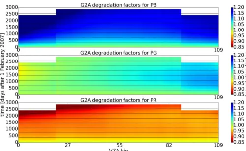
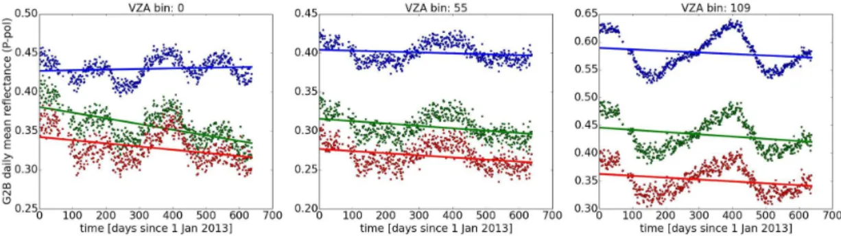
to a VZA. The 192 PMD pixel of the full 1920 km swath are mapped to 110 viewing zenith angle bins of one degree width, which covers the region from−55◦ (east edge of swath) to+₅₅◦_{(west edge of swath) in VZA. Each global daily mean reflectance is} comprised of all measurements within the latitude range from 60◦N to 60◦S. For the whole data baseline, examples of the temporal evolution of the GOME-2A degradation

5

are shown in Fig. 1 for the colors PB, PG and PR for three selected VZA bins: VZA bin 0 (east edge of swath, VZA [−55,−50]◦), VZA bin 55 (nadir part of swath, VZA [0, 5]◦) and VZA bin 109 (west edge of the swath, VZA [50, 55]◦). The same is shown for GOME-2B in Fig. 3.

Short term periodic components in both cases are interpreted as variations due

10

to seasonal changes, e.g. seasonal changes in snow and ice coverage, vegetation, foilage etc. (all resulting from Earth’s obliquity against the orbital plane). In contrast, the long term component in both cases, GOME-2A and GOME-2B, is addressed to instrumental degradation. For GOME-2A we chose a polynomial component of third degree and for GOME-2B a linear component (linear instead of 3rd degree because

15

the GOME-2B data only cover one and a half years and a 3rd order polynomial would also fit the seasonal component).

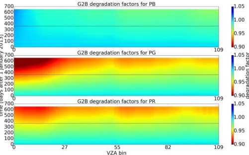
We calculate degradation factors as a function of time and VZA by normalizing the polynomial (GOME-2A) or linear (GOME-2B) component to the reference measure-ments from 1 February 2007 for GOME-2A and 1 January 2013 for GOME-2B. Further,

20

correction factors to be multiplied with the reflectances are calculated as the inverse of the degradation factors and stored in look-up tables (LUTs). The degradation fac-tors for GOME-2A and GOME-2B are shown in Figs. 2 and 4. It is obvious that the degradation of the reflectances does not follow a similar pattern but instead strongly depends on wavelength range (OCRA color) and viewing zenith angle. Also, depending

25

on the degradation in the Solar port compared to the Earth port, the degradation of the reflectance can be positive or negative.

(9)

AMTD

8, 13471–13524, 2015

R. Lutz et al.

Title Page

Tables Figures

◭ ◮

Back Close

Full Screen / Esc

Discussion

P

a

per

|

Discussion

P

a

per

|

Discussion

P

a

per

|

Discussion

P

a

per

|

for the three OCRA colors PB (Fig. 5), PG (Fig. 6) and PR (Fig. 7) for the PMD pixels 0 (east edge of swath, top panel), 95 (near nadir, middle panel) and 191 (west edge of swath, bottom panel). The reference measurement for GOME-2A is 1 February 2007 (MetOp-A orbit 1483) and for GOME-2B 1 January 2013 (MetOp-B orbit 1497), re-sulting in a similar in-orbit time at the reference points. The time diff_{erence between}

5

the two reference points for GOME-2A and GOME-2B is 2161 days. The colored dots represent GOME-2A data while the black dots represent GOME-2B data in the same timeline as GOME-2A, i.e. the GOME-2B timeline plus 2161 days. The grey circles rep-resent GOME-2B data shifted such that they can be compared to the initial degradation of GOME-2A. The left dashed line marks the transition from PMD Def v1.0 to PMD Def

10

v3.1 on 12 March 2008 for GOME-2A (which mainly aff_{ects PB, but to a neglibile} ex-tend PG and PR) and the right dashed line represents the FM3 key data upgrade for MetOp-A on 3 July 2012, which does not seem to aff_{ect any of the colors.}

The left hand side of the figures allows to estimate the eff_{ect of the PMD Definition} version on the RGB reflectances. Left to the dashed line, PMD Def v1.0 was used

15

for GOME-2A and right to the dashed line PMD Def v3.1 was applied for GOME-2A. The eff_{ect is significant for PB while it is minor for PG and PR. Also, the GOME-2B} reflectances shifted to match the in-orbit time of GOME-2A align very well with the GOME-2A reflectances after 12 March 2008. This is because the PMD Definitions for GOME-2B are very close to the PMD Def v3.1 of GOME-2A.

20

The right hand side of the figures allows to estimate the eff_{ect of degradation and} demonstrates that it is non-trivial but instead depends not only on time but also on wavelength range (here color PB, PG or PR) and viewing zenith angle (here PMD pixels 0, 95 and 191).

2.3.2 Dependencies on viewing angles, latitudes and seasons 25

(10)

AMTD

8, 13471–13524, 2015

R. Lutz et al.

Title Page

Tables Figures

◭ ◮

Back Close

Full Screen / Esc

Discussion

P

a

per

|

Discussion

P

a

per

|

Discussion

P

a

per

|

Discussion

P

a

per

|

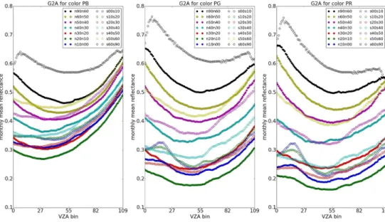
9 for GOME-2A and GOME-2B, respectively). We consider a total of 14 latitude bands. Twelve bands with a width of 10◦between [−60,+_{60] and a two bands with a width of} 30◦ for latitudes>60 and<−60 (i.e. towards the poles). To estimate the eff_{ect of the} viewing angle and the latitude on the measured mean reflectance, and to statistical soft correct for it, we do the following procedure for each month considered. For each PMD

5

pixelx the mean reflectance of every latitude band ¯ϕis calculated for a whole month of data and fitted with a fourth order polynomial:

ρmean(x, ¯ϕ)=αx, ¯ϕ+βx, ¯ϕ·x+γx, ¯ϕ·x2+δx, ¯ϕ·x3+ǫx, ¯ϕ·x4, (2)

whereα_x, ¯ϕ,βx, ¯ϕ,γx, ¯ϕ,δx, ¯ϕ andǫx, ¯ϕ are the fit parameter for the corresponding pixel

x (PMD pixels from 0 to 191) and latitude band ¯ϕ. The correction factor c(x, ¯ϕ) for

10

the reflectance measurement at pixelx and latitude band ¯ϕ is calculated by normal-ization to the mean reflectance of the close-to-nadir pixel (PMD pixel 95 of 191) of the corresponding latitude band:

c(x, ¯ϕ)= ρmean(x, ¯ϕ)

ρmean(95, ¯ϕ)

(3)

To get the correction factorc(x,ϕ) for an arbitrary latitudeϕ, we apply a linear spline

15

interpolation between the correction factorsc(x, ¯ϕ) of the 14 latitude bands ¯ϕfor each of the across-track PMD pixelsx. If the VZA is used instead of the across-track PMD pixel position, thex in Eqs. (2) and (3) has to be replaced by the VZA and the nadir pixel 95 in the denominator of Eq. (3) has to be replaced by the VZA bin 55 which is the VZA bin closest to nadir.

20

For each month considered, the fitting parameter to calculate the pixel- and latitude dependent correction values for all OCRA colors and polarisations are then stored in LUTs. The same is done in the case of the VZA- and latitude dependent correction values. The viewing angle and latitudinal dependency for GOME-2A is shown for the example of the month February 2007 for the P pol data in Fig. 8 and for GOME-2B for

25

(11)

AMTD

8, 13471–13524, 2015

R. Lutz et al.

Title Page

Tables Figures

◭ ◮

Back Close

Full Screen / Esc

Discussion

P

a

per

|

Discussion

P

a

per

|

Discussion

P

a

per

|

Discussion

P

a

per

|

As can be seen as a general feature, for all three colors the monthly mean reflectances are larger at the swath edges than at the nadir position or, more generally, at the central part of the swath. Similarly, the monthly mean reflectances are larger in polar and sub-polar latitudes and smaller in tropical latitudes. Also the curvature is slightly diff_erent in diff_{erent months throughout the year. It seems to be stronger in winter months and}

5

flatter in summer months (not shown here).

Similar to the degradation correction, the correction factors for the dependencies on viewing angles, latitudes and seasons are also stored in LUTs for all combinations of colors and polarization state. See Fig. 10 for the temporal evolution of the correction factors for viewing angle and latitudinal dependencies for GOME-2A (February 2007

10

until September 2014) and GOME-2B (January 2013 until September 2014), respec-tively. The annual periodicity is clearly visible.

2.4 Construction of cloud-free reflectance composites

After correcting the reflectances for instrumental degradation and dependencies on viewing angles, latitudes and seasons, we apply the following color approach to

deter-15

mine cloud-free reflectance composite maps.

First, a grid with a resolution of 0.2◦ in latitude and longitude is defined (globally re-sulting in 900×1800=_{1 620 000 grid cells)}1_{. For each grid cell we collect all GOME-2A} measurements between April 2008 and June 2013 (63 months), whose central longi-tude and latilongi-tude are within the borders of each grid cell. Since we want to derive

20

monthly cloud-free composites, these measurements are further divided according to the month in which they were taken (the same months in consecutive years are com-bined). Based on the 5 years dataset, the resulting number of measurements per grid cell and per month is around 120 to 180, depending on the geolocation. For each color

1

(12)

AMTD

8, 13471–13524, 2015

R. Lutz et al.

Title Page Abstract Introduction Conclusions References Tables Figures ◭ ◮ ◭ ◮ Back Close

Full Screen / Esc

Printer-friendly Version Interactive Discussion Discussion P a per | Discussion P a per | Discussion P a per | Discussion P a per |

(PB, PG and PR) the normalized color (Pb, Pg and Pr) is obtained via

Pb= PB

PB+_PG+_PR (4a)

Pg= PG

PB+_PG+_PR (4b)

Pr= PR

PB+_PG+_PR (4c)

The normalized colors based on S polarization (Sb, Sg and Sr) are obtained in a

sim-5

ilar way. In a Pr-Pg or Sr-Sg color diagram, let w=₍1 3,

1

3) be the white point and

MP=(Pr, Pg) and MS=(Sr, Sg) be the measurements based on P polarization and S polarization, respectively. Then the distancesdPanddSfrom the mesurement to the white point for the two polarization cases are given by

dP= s

Pr−1

3 2

+

Pg−1

3 2

, (5a)

10

dS= s

Sr−1

3 2

+

Sg−1

3 2

(5b)

The distances from the white point are calculated for all measurements within a grid cell and the RGB colors of the measurement with the largest distance from the white point is defined to represent the cloud-free situation of that grid cell. By merging the cloud-free condition of all grid cells, we can finally obtain global cloud-free TOA

re-15

flectance composite maps for each month and RGB color. All cloud-free composite maps are stored in Look-up tables. Some examples for the spring and summer months for color B (P pol based) are shown in Fig. 11. Close to the poles it may occur that cells do not contain enough data. Such cells are assigned with nan-values and appear grey in the plots. Since a proper construction of the cloud-free composites requires a large

20

(13)

AMTD

8, 13471–13524, 2015

R. Lutz et al.

Title Page

Tables Figures

◭ ◮

Back Close

Full Screen / Esc

Discussion

P

a

per

|

Discussion

P

a

per

|

Discussion

P

a

per

|

Discussion

P

a

per

|

for creating the cloud-free maps. The current GOME-2B data record is yet well below three years and simply too short to achieve enough measurements per grid cell to de-rive stable cloud-free values at the given grid cell resolution of 0.2 by 0.2◦. Once the mission lifetime of GOME-2B will be above four to five years, we will create cloud-free composites based on the GOME-2B data themselves to derive the GOME-2B OCRA

5

cloud fractions. Until then, the GOME-2A maps will be used for GOME-2B too. Fig-ure 12 shows rg-diagrams of the yearly temporal evolution of the cloud-free conditions for six diff_{erent surface types. It can be nicely seen that the cloud-free background does} not change significantly for the Amazonas, South Atlantic and Sahara cases throughout the course of the year. In contrast, the Vancouver, Alpes and Hudson Bay cases show

10

significant monthly changes of the cloud-free background during the melting season (April–May–June) and the beginning of winter with fresh snow (October–November– December). Also, fresh snow seems to have lower Pr values (November, December) compared to old snow (March).

2.5 Cloud fraction determination 15

The determination of the radiometric cloud fraction with OCRA follows a two-step pro-cess. The first part consists of the separation of a scene into a contribution from the clouds and a cloud-free background and has been described in Sect. 2.4. The second part performs a comparison of the measured reflectance of a scene with its corre-sponding cloud-free situation. This second step is now outlined in the following

sub-20

subsections.

2.5.1 Matching the measurements to the cloud-free grid

In order to find the corresponding cloud-free reflectance to a measured scene, we search for the grid cell of the composite map which contains the central latitude and longitude of the measured pixel. The final cloud-free value is determined via linear

25

(14)

ob-AMTD

8, 13471–13524, 2015

R. Lutz et al.

Title Page

Tables Figures

◭ ◮

Back Close

Full Screen / Esc

Discussion

P

a

per

|

Discussion

P

a

per

|

Discussion

P

a

per

|

Discussion

P

a

per

|

servation. We assume a monthly cloud-free map to correspond to the middle of the month. If a measurement is dated in the first half of a month, we find the cloud-free value via linear interpolation between the cloud-free maps of the previous and current month and if the measurement is dated in the second part of a month, we obtain the cloud-free value via linear interpolation between the cloud-free maps of the current and

5

next month.

2.5.2 OCRA

OCRA determines the cloud fraction using the diff_{erences between the colors of a} mea-sured scene and its corresponding cloud-free values. Letρ(λi), withi=R, G, B, be the

measured reflectances and ρCF(λi) the cloud-free background values of the grid cell 10

corresponding to the geolocation of the measured reflectances. The radiometric cloud fractionfcis then obtained by the following equation

fc=min (

1, v u u t

X

i=R,G,B

α(λi)·max

n

0,ρ(λi)−ρCF(λi)−β(λi)

o2)

, (6)

where the scaling factorsα(λi) are determined by a histogram analysis of the difference

ρ(λ_i)−ρCF(λi) at a cumulative histogram value of 0.99 as 15

α(λi)=

1

(ρ(λ_i)−ρCF(λi))20.99

(7)

and the off_{set values} _β₍_λ_i_{) are determined by a histogram analysis of the di}ff_erence

ρ(λ_i)−ρCF(λi) at the mode of the normal histogram as

β(λi)=(ρ(λi)−ρCF(λi))mode. (8) These parametersαandβpractically act as upper and lower thresholds defining a fully

20

(15)

AMTD

8, 13471–13524, 2015

R. Lutz et al.

Title Page

Tables Figures

◭ ◮

Back Close

Full Screen / Esc

Discussion

P

a

per

|

Discussion

P

a

per

|

Discussion

P

a

per

|

Discussion

P

a

per

|

shadowing eff_{ects, darkening due to aerosols). The max(0,}_x_{) and min(1,}_x_{) functions} in the equation above ensure a mapping of the cloud fractions to the interval [0, 1].

The cloud fraction determination is done separately for the P based colors (PB, PG, PR) and S based colors (SB, SG, SR) and the final cloud fraction is taken as the mean of the P and S based cloud fractions.

5

For GOME-2A the scaling factorsα and off_{set values}_β_{are determined from 29 test} days spread over a 6 year period. Each test day uses the same criteria: the scaling factor α via the 0.99 cumulative histogram value of the diff_erence _ρ₍_λ_i₎₋_ρ_CF₍_λ_i_{) and} the off_{set value}_β_{via the mode of the normed histogram value of}_ρ₍_λ

i)−ρCF(λi). See

Fig. 13 for an example. Over the 6 year time base, there is no significant trend or

10

variation seen in the parameters of the 29 test days, hence we can use one fixed set of alphas and betas for the whole mission (see Table 3). For GOME-2B we use 6 test days spread over a time period of 18 months to determine the scaling factors and off_set values.

An example of a normalized rg-color diagram for a grid cell near Munich for the month

15

April is shown in Fig. 14 and contains 128 measurements which happend to be in this grid cell in the month April during the years 2007 to 2013. It is obvious that the strong variation of the cloud-free condition from one month to the other (big star symbols in the plot) call for an interpolation towards daily cloud-free values (small star symbols in the plot).

20

2.6 Sun glint removal

Under certain geometrical conditions it may happen that sunlight reflected by the ocean surface directly reaches the satellite sensor, enhancing the measured signal in com-parison to a non-aff_{ected scene over water. This e}ff_{ect is called sun glint. More details} on this eff_{ect may be found in Kay et al. (2009, 2013). Since clouds in the visual appear}

25

(16)

MetOp-AMTD

8, 13471–13524, 2015

R. Lutz et al.

Title Page

Tables Figures

◭ ◮

Back Close

Full Screen / Esc

Discussion

P

a

per

|

Discussion

P

a

per

|

Discussion

P

a

per

|

Discussion

P

a

per

|

A/B orbits, sun glint for GOME-2 can only appear in the east part of the swath. Based on the Solar zenith angleΘ

⊙, satellite zenith angle Θsat, Solar azimuth angleϕ⊙ and satellite azimuth angleϕsat, a sunglint factorνis calculated:

ν= q

(|Θ

⊙−Θsat| −2)2+(ϕsat−ϕ⊙−180)2 (9) OCRA raises a flag of possible sun glint ifνis below a certain thresholdνthreswhich was

5

determined empirically and set to 25, and if the measurement is over water. For each orbit, this results in roughly ellipsoidal shaped regions in the eastern part of the swath which have an extension of roughly 30◦ in latitudinal and 10◦ in longitudinal direction. The possibility for sun glint increases the closer the measurement is to the center of the ellipse. This is illustrated in Fig. 15. The latitudinal location of the ellipse depends

10

on the season and reaches its highest latitudes in June/July, extending roughly from +_{60 to}+₂₀◦_{. The lowest latitudes are reached in December/January, extending roughly} from 0 to−40◦.

Based on Loyola et al. (2011), in addition to flagging possible sun glint situations, we also improved the algorithm to find a correction for the aff_{ected scenes. To do so, we}

15

need to distinguish if a retrieved cloud fraction is in fact due a cloud or if it is mimicked by sun glint (which can only appear in the abscence of clouds under clear sky conditions). For measurements which may possibly be aff_{ected by sun glint and also are over water,} the following steps are undertaken. First we consider a cloud fraction threshold of 0.1. Sun glint is only corrected for above this threshold, meaning that we assume sun glint

20

to cause cloud fraction signals above 0.1. Next, we introduce three quantities which are capable to distinguish clouds from sun glint if they are used in concert. One is a reflectance ratio in the blue spectral part. We use the ratio of PMD4 to PMD3 (see Table 1). The second is the Stokes fraction (see Sect. 3.7 in Munro et al., 2015 for further information) in the red (PMD12) and the third is the ratio of the OCRA colors

25

(17)

AMTD

8, 13471–13524, 2015

R. Lutz et al.

Title Page

Tables Figures

◭ ◮

Back Close

Full Screen / Esc

Discussion

P

a

per

|

Discussion

P

a

per

|

Discussion

P

a

per

|

Discussion

P

a

per

|

help to distinguish clouds from sun glint. If the absolute value of Stokes12 is below a certain threshold, the signal will be due to clouds and cannot be due to sun glint. This is based on the assumption that clouds tend to be de-polarizing due to multiple scattering and the Stokes fraction will therefore be close to zero for cloudy scenes. A detailed investigation of GOME-2 polarization spectra and the influence of clouds

5

on the Stokes fraction is presented in Tilstra et al. (2014a). Finally, if the value of the third indicator PRPB is below a certain threshold, the signal will be likely due to a cloud because sun glint would result in a signal well above this threshold. Thus combining these three criteria, we are able to distinguish between cloud and sun glint, and hence correct for it (the cloud fraction is set to zero in this case). The three quantities used in

10

our sun glint removal procedure are shown together with the cloud fractions before and after sun glint removal for a test scene in Fig. 16. Note that the bright ellipsoidal sun glint signals are successfully removed in the bottom middle panel without aff_{ecting the} true cloud signals. The empirical thresholds are PSG=_{1.050, abs(Stokes12)}=_0.125 and PRPB=_{1.15 for GOME-2A data before 11 March 2008 (i.e. valid for PMD Def. 1.0),}

15

PSG=_{1.080, abs(Stokes12)}=_{0.125 and PRPB}=_{1.15 in the case of GOME-2A data} after 11 March 2008 (i.e. valid for PMD Def. 3.1) and PSG=_{0.995, abs(Stokes12)}=_0.1 and PRPB=_{1.0 in the case of GOME-2B. A flag is set for each measurement where} a sunglint correction was applied (see bottom right panel in Fig. 16). For all quantities involved, we use the corrected reflectances as outlined in Sect. 2.3.

20

A similar approach to investigate sun glint in GOME-2 data has already been pre-sented by Loyola et al. (2011) and Beierle et al. (2013).

An example for a full day of OCRA cloud fractions after sun glint filtering, based on GOME-2A and GOME-2B data merged together, is shown in Fig. 17.

2.7 Comparison of cloud fractions from GOME-2A and GOME-2B 25

(18)

AMTD

8, 13471–13524, 2015

R. Lutz et al.

Title Page

Tables Figures

◭ ◮

Back Close

Full Screen / Esc

Discussion

P

a

per

|

Discussion

P

a

per

|

Discussion

P

a

per

|

Discussion

P

a

per

|

possible similar geographic coverage is established. Figure 18 shows the monthly mean cloud fractions for GOME-2A and GOME-2B, subdivided in ten degree wide zonal bins (left panel) and thirty degree wide meridional bins (right panel). The green solid line represents the original GOME-2B data while the red solid line is based on GOME-2B reflectances homogenized to the GOME-2A reflectances. This shift of the

5

GOME-2B reflectances was performed in order to match the GOME-2A reflectances as good as possible and is based on 30 full days of data. Figure 19 shows the correlation of the cloud fraction data mentioned above for the cases based on original GOME-2B reflectances (y axis in left panel) and homogenized GOME-2B reflectances (y axis in right panel).

10

3 Comparison with AVHRR data

We compared twelve days of OCRA data from GOME-2A/B with data from the AVHRR (Advanced Very High Resolution Radiometer) instrument, which is mounted on the same platform as the GOME-2 instruments, i.e. on MetOp-A and MetOp-B. AVHRR is an across track scanner sensing the radiation backscattered from Earth in six channels

15

from the visible/near infrared range towards the thermal infrared. The spatial resolution is 1 km at nadir. Based on the dedicated cloud-test results provided with the AVHRR level-1B files, the geometrical cloud fraction for one GOME-2 PMD pixel is derived as the fraction of the sum of all cloudy pixels to the total number of AVHRR pixels collo-cated within one GOME-2 PMD pixel. This AVHHR cloud fraction is then added as an

20

extra field to the GOME-2 level-1B file. We have been provided with twelve test days of collocated AVHRR geometrical cloud fractions to GOME-2 PMD pixels2. These com-prise the first day of each month between December 2012 and November 2013. Here we compare the GOME-2A OCRA radiometric cloud fractions for 1 December 2012 with the collocated AVHRR geometrical cloud fractions. Figure 20 shows the OCRA

25

2

(19)

AMTD

8, 13471–13524, 2015

R. Lutz et al.

Title Page

Tables Figures

◭ ◮

Back Close

Full Screen / Esc

Discussion

P

a

per

|

Discussion

P

a

per

|

Discussion

P

a

per

|

Discussion

P

a

per

|

(top left) and AVHRR (bottom left) cloud fractions for MetOp-A on a world map. The absolute diff_{erences are plotted in the top right and a correlation map is found on the} bottom right. The overall large-scale cloud structures are very similar in both prod-ucts. Although the linear correlation is relatively high (linear correlation coeffi_{cient of} 0.88, see bottom right panel), diff_{erences appear as a systemetac o}ff_{set towards larger}

5

AVHRR cloud fractions of roughly 0.16. This may be explained by the fact that UVN ra-diances from GOME-2 are not sensitive to clouds with low optical thickness, e.g. cirrus clouds, whereas the IR or thermal infrared radiances from AVHRR are. In Fig. 21, his-tograms of the cloud fractions based on OCRA and AVHRR are plotted in the left panel. The right panel shows a histogram of the cloud fraction diff_{erences between OCRA and}

10

AVHRR for the same day (1 December 2012). The histogram of the cloud fraction dif-ferences has a mean and a standard deviation of−0.15 and 0.20, respectively, and looks very similar to the histogram shown in the right panel of Fig. 4 in Loyola et al. (2007). The latter compares OCRA cloud fractions derived from the GOME (Global Ozone Monitoring Experiment) instrument on ERS-2 (European Remote Sensing 2

15

Satellite) and the SEVIRI (Spinning Enhanced Visible and Infrared Imager) instrument on MSG (METEOSAT Second Generation) and finds a mean diff_{erence of}₋_{0.21 with} a standard deviation of 0.26. Since GOME is not sensitive to optically thin clouds, but SEVIRI is, the situation is very similar to the comparison of the GOME-2/AVHRR pair. One possibility to circumvent these diff_{erent cloud sensitivities and to achieve a better}

20

agreement is to filter clouds with low optical thickness (below a certain threshold) from the AVHRR or SEVIRI data. For the latter case this has been done in the left panel of Fig. 4 by Loyola et al. (2007) and results in a much better agreement of the GOME and SEVIRI data. Concerning GOME-2 and AVHRR, a similar cloud optical thickness filtering of the AVHRR data is outlined in the following subsection.

25

3.1 Cloud optical thickness filter

(20)

EU-AMTD

8, 13471–13524, 2015

R. Lutz et al.

Title Page

Tables Figures

◭ ◮

Back Close

Full Screen / Esc

Discussion

P

a

per

|

Discussion

P

a

per

|

Discussion

P

a

per

|

Discussion

P

a

per

|

METSAT Polar multi-sensor Aerosol product (PMAP) additionally to the cloud fraction also provides the cloud optical depth (COD). Further details can be found in the PMAP Factsheet EUMETSAT (2015).

A comparison of the OCRA cloud fractions to the AVHRR cloud fractions taken from this PMAP product is shown in Fig. 22 for data from 1 May 2014. Both dataset are

5

matched to a common lat/lon grid of 0.4◦resolution. As before, the general large-scale cloud structures agree very well. To account for GOME-2 insensitivity to low optical thickness clouds, we filtered out all AVHRR cloud fraction measurements which have a COD smaller than 5. Additionally, all cloud fractions larger than 0.95 are rejected in order to avoid ambiguities due to diff_{erent treatment of the cloud fraction over snow/ice}

10

scenes, where the AVHRR cloud fraction is set to 1. The eff_{ect of this treatment is} visible in Fig. 23. Note that in the top left panel there are many CF=_{1 cases for AVHRR} which are considerably less for OCRA. The major contribution to these large deviations comes from polar regions (this is also obvious in Fig. 22). In the histograms of the cloud fractions (top panels) and histograms of the cloud fraction diff_{erences (bottom panels)}

15

visualized in Fig. 23 it is noted that the COD and CF filtering is able to remove the strong assymmetry seen in the bottom left panel, but the rather large systematic off_{set (}₋_0.24 in this case) still remains in the bottom right panel. Finally, Fig. 24 nicely illustrates that this systematic off_{set between the radiometric (GOME-2) and the geometric (AVHRR)} cloud fractions is more or less constant over the whole latitude range.

20

Most plots in the previous sections are only shown for reflectances based on the P pol PMD data. Only in the final cloud fraction map, Fig. 17, the mean of the P pol based and S pol based data are used. Larger discrepancies between the two polar-ization states may appear for instrumental degradation and scan angle dependencies. Since these latter eff_{ects are corrected for during the reflectance normalization, the}

25

(21)

AMTD

8, 13471–13524, 2015

R. Lutz et al.

Title Page

Tables Figures

◭ ◮

Back Close

Full Screen / Esc

Discussion

P

a

per

|

Discussion

P

a

per

|

Discussion

P

a

per

|

Discussion

P

a

per

|

4 Cloud fraction over snow/ice conditions

A known issue for cloud fraction retrieval algorithms in the UVN wavelength range is the performance over very bright surfaces like snow or ice. In such cases, often external databases of daily snow/ice cover are incorporated and the aff_{ected scenes are flagged} and given an arbitrary cloud fraction value, e.g. 1, and an eff_{ective scene albedo is}

re-5

trieved instead. In OCRA, the cloud fraction is calculated regardless of the surface condition. For the snow/ice scenes mentioned above, this requires the cloud-free back-ground maps to be as close as possible to the current surface situation in order to represent the cloud fraction over snow/ice as realistically as possible. As mentioned before, the cloud-free reflectances for the OCRA RGB colors of a particular grid cell

10

are interpolated towards a daily value in between two monthly cloud-free maps. If we imagine that the cloud-free reflectance of a particular grid cell represents a snow/ice situation (i.e. higher background) and in the same cell the snow/ice is melted in the next month (i.e. lower background), OCRA’s linear interpolation scheme may intro-duce some uncertainties since snow/ice melting and particularly new snow/ice

cover-15

age may happen on shorter timescales than 30 days. If melting or new snow occurs in the timescale of days, it would of course be better to have e.g. weekly cloud-free maps, but for this there are simply not enough data available. Hence, monthly maps with linear interpolation is the best tradeoff_{that can be done given the current} combi-nation of timebase, grid cell size and PMD pixel size. The eff_{ect of melting seasons and}

20

fresh snow coverage on the cloud-free backgound was shown in Fig. 12. In this figure, it can also be seen that even for snow/ice surfaces the cloud-free background does not coincide with the white point of the rg-diagram, which is why OCRA can also retrieve the cloud fraction for these cases instead of setting an arbitrary value. However, OCRA may slightly underestimate the cloud fraction in these cases due to the fact that the

25

(22)

AMTD

8, 13471–13524, 2015

R. Lutz et al.

Title Page

Tables Figures

◭ ◮

Back Close

Full Screen / Esc

Discussion

P

a

per

|

Discussion

P

a

per

|

Discussion

P

a

per

|

Discussion

P

a

per

|

conditions), but in this case it might be worthwile to consider having separate scaling factors for the diff_{erent surface types (e.g. permanent ice, sea ice, snow, desert,} wa-ter, land). Surface dependent scaling factors will be included in a future update to the OCRA algorithm.

An alternative to choosing the maximum distance in the rg-diagram as the cloud-free

5

situation would be to do a histogram analysis ofρ(λ_i)−ρCF(λi) for each individual grid

cell. This would work fine for gaussian distributions (grid cells without strong surface condition variations) but would also cause problems if the distribution is bimodal or multimodal (grid cells with seasonal changes of the surface conditions).

Further attempts have been undertaken in order to distinguish snow/ice from clouds.

10

It was noticed that the diff_{erence between the P pol based OCRA cloud fraction and the} S pol based OCRA cloud fraction depends slightly on the underlying surface. As can be seen in the right panel of Fig. 25, the cloud fraction diff_{erence of the P pol based cloud} fraction minus the S pol based cloud fraction seems to be particularly negative (blue in the plot) over snow/ice covered surfaces, e.g. Antarctica, Hudson Bay, Greenland,

15

Siberia. Being an interesting aspect, this approach to identify snow/ice via the cloud fractions based on diff_{erent polarisation states may be pursued further in future work.}

Another approach to tackle the snow/ice issues and to discriminate snow/ice sur-faces from clouds was presented by Zhang and Xiao (2014) for images with very high spatial resolution. We tried to adapt this method to the GOME-2 PMD footprints which

20

have a much smaller spatial resolution. The basic idea is to convert the RGB color infor-mation to a HSI (Hue, Saturation, Intensity) color space. Since clouds have high inten-sitiesIbut low saturationsS, a map of the significanceW =_I/S _{can clearly distinguish} clouds from non-cloudy surfaces. However, especially over the regions of interest, i.e. snow/ice, it was not able to derive satisfactorily stable and robust thresholds to include

25

(23)

AMTD

8, 13471–13524, 2015

R. Lutz et al.

Title Page

Tables Figures

◭ ◮

Back Close

Full Screen / Esc

Discussion

P

a

per

|

Discussion

P

a

per

|

Discussion

P

a

per

|

Discussion

P

a

per

|

5 Conclusions

In this paper we have presented version 3.0 of the OCRA cloud fraction algorithm ap-plied to data measured with the GOME-2 instrument onboard the MetOp satellites. Improvements with regard to the previous OCRA version include a degradation correc-tion of the PMD reflectances as well as correccorrec-tions for scan angle dependencies and

5

latitudinal dependencies. In addition, the cloud-free composite maps are now based on more than six years of GOME-2A data. An improved sun glint flagging and removal has been implemented, which now also considers the Stokes fraction and an additional color ratio in order to distinguish between sun glint and real clouds.

The PMD based OCRA cloud fractions have been compared to collocated AVHRR

10

cloud fractions and show a good general agreement. However, a systematic off_{set is} addressed to diff_{erent sensitivities to low optical thickness clouds due to the di}ff_erent spectral ranges covered by the GOME-2 and AVHRR instruments.

In addition to the simple OCRA color space approach, which does not need ex-pensive radiative transfer modelling, another advantage of OCRA lies in its extremely

15

fast computational performance. This is especially relevant for providing products in near real time. All external input, like the cloud free reflectance composite maps, are pre-calculated look-up tables (LUTs) and do not need to be calculated online. The radiometric cloud fractions for a full GOME-2 orbit with around 120 000 single PMD measurements are calculated in only ≈20 s (operational). The OCRA algorithm was

20

used for the generation of operational products from GOME and SCIAMACHY and is not limited to PMD data, but can also be used with normal radiance data (e.g. OMI, TROPOMI). At the beginning of a new mission, cloud-free reflectance composites from a predecessor mission can be used as an initial input until enough data are collected to produce cloud-free reflectance composite maps based on the same instrument.

25

(24)

AMTD

8, 13471–13524, 2015

R. Lutz et al.

Title Page

Tables Figures

◭ ◮

Back Close

Full Screen / Esc

Discussion

P

a

per

|

Discussion

P

a

per

|

Discussion

P

a

per

|

Discussion

P

a

per

|

The article processing charges for this open-access publication were covered by a Research Centre of the Helmholtz Association.

References

Beierle, S., de Vries, M., Lang, R., and Wagner, T.: An empirical Sun-glint index for GOME-2, 2013 Joint EUMETSAT/AMS Conference, 16–20 September 2013,

Vi-5

enna, Austria, available at: http://www.eumetsat.int/website/wcm/idc/idcplg?IdcService=

GET_FILE&dDocName=_{PDF_CONF_P_S6_01_BEIRLE_P&RevisionSelectionMethod}=

LatestReleased&Rendition=_{Web (last access: 18 December 2015), 2013. 13487}

Burrows, J. P., Weber, M., Buchwitz, M., Rozanov, V., Ladstätter-Weißenmayer, A., Richter, A., Debeek, R., Hoogen, R., Bramstedt, K., Eichmann, K.-U., Eisinger, M., and Perner, D.: The

10

Global Ozone Monitoring Experiment (GOME): mission concept and first scientific results, J. Atmos. Sci., 56, 151–175, 1999. 13474

Dobber, M. R., Dirksen, R. J., Levelt, P. F., van den Oord, G. H. J., Voors, R. H. M., Kleipool, Q., Jaross, G., Kowalewski, M., Hilsenrath, E., Leppelmeier, G. W., de Vries, J., Dierssen, W., and Rozemeijer, N. C.: Ozone monitoring instrument calibration, IEEE T. Geosci. Remote,

15

44, 1209–1238, 2006. 13474

EUMETSAT: GOME-2 Factsheet, available at: http://www.eumetsat.int/website/wcm/idc/idcplg? IdcService=_{GET_FILE&dDocName}=_{PDF_GOME_FACTSHEET&RevisionSelectionMethod} =_{LatestReleased&Rendition}=_{Web (last access: 18 December 2015), 2014. 13474, 13497}

EUMETSAT: PMAP Factsheet, available at: http://www.eumetsat.int/website/wcm/idc/idcplg?

20

IdcService=_{GET_FILE&dDocName}=_{PDF_PMAP_FACTSHEET&RevisionSelectionMethod} =_{LatestReleased&Rendition}=_{Web, 2015. 13490}

Grzegorski, M., Wenig, M., Platt, U., Stammes, P., Fournier, N., and Wagner, T.: The Heidelberg iterative cloud retrieval utilities (HICRU) and its application to GOME data, Atmos. Chem. Phys., 6, 4461–4476, doi:10.5194/acp-6-4461-2006, 2006. 13474

25

(25)

AMTD

8, 13471–13524, 2015

R. Lutz et al.

Title Page

Tables Figures

◭ ◮

Back Close

Full Screen / Esc

Discussion

P

a

per

|

Discussion

P

a

per

|

Discussion

P

a

per

|

Discussion

P

a

per

|

Kay, S., Hedley, J., and Lavender, S.: Sun glint estimation in marine satellite images: a compar-ison of results from calculation and radiative transfer modeling, Appl. Optics, 52, 5631, 2013. 13485

Kokhanovsky, A. A., Rozanov, V. V., Zege, E. P., Bovensmann, H., and Burrows, J. P.: A semi-analytical cloud retrieval algorithm using backscattered radiation in 0.4–2.4 µm spectral

re-5

gion, J. Geophys. Res.-Atmos., 108, AAC 4-1–AAC 4–19, doi:10.1029/2001JD001543, 2003. 13474

Levelt, P. F., van den Oord, G. H. J., Dobber, M. R., Malkki, A., Visser, H., de Vries, J., Stammes, P., Lundell, J. O. V., and Saari, H.: The Ozone Monitoring Instrument, IEEE T. Geosci. Remote, 44, 1093–1101, 2006. 13474

10

Loyola, D.: A new cloud recognition algorithm for optical sensors, Int. Geosci. Remote Se., 2, 572–574, 1998. 13474

Loyola, D.: Automatic cloud analysis from polar-orbiting satellites using neural network and data fusion techniques, Int. Geosci. Remote Se., 4, 2530–2533, 2004. 13474

Loyola, D., Thomas, W., Livschitz, Y., Ruppert, T., Albert, P., and Hollmann, R.: Cloud properties

15

derived from GOME/ERS-2 backscatter data for trace gas retrieval, IEEE T. Geosci. Remote, 45, 2747–2758, 2007. 13489

Loyola, D. G., Koukouli, M. E., Valks, P., Balis, D. S., Hao, N., Van Roozendael, M., Spurr, R. J. D., Zimmer, W., Kiemle, S., Lerot, C., and Lambert, J.-C.: The GOME-2 total column ozone product: Retrieval algorithm and ground-based validation, J. Geophys.

Res.-20

Atmos., 116, d07302, doi:10.1029/2010JD014675, 2011. 13486, 13487

Munro, R., Lang, R., Klaes, D., Poli, G., Retscher, C., Lindstrot, R., Huckle, R., Lacan, A., Grzegorski, M., Holdak, A., Kokhanovsky, A., Livschitz, J., and Eisinger, M.: The GOME-2 instrument on the Metop series of satellites: instrument design, calibration, and level 1 data processing – an overview, Atmos. Meas. Tech. Discuss., 8, 8645–8700,

doi:10.5194/amtd-25

8-8645-2015, 2015. 13473, 13486

Schoeberl, M. R., Douglass, A. R., Hilsenrath, E., Bhartia, P. K., Beer, R., Waters, J. W., Gun-son, M. R., Froidevaux, L., Gille, J. C., Barnett, J. J., Levelt, P. F., and de Cola, P.: Overview of the EOS Aura Mission, IEEE T. Geosci. Remote, 44, 1066–1074, 2006. 13474

Tilstra, L. G., Tuinder, O. N. E., and Stammes, P.: A new method for in-flight degradation

correc-30

(26)

AMTD

8, 13471–13524, 2015

R. Lutz et al.

Title Page

Tables Figures

◭ ◮

Back Close

Full Screen / Esc

Discussion

P

a

per

|

Discussion

P

a

per

|

Discussion

P

a

per

|

Discussion

P

a

per

|

September 2012, Sopot, Poland, available at: http://www.temis.nl/airpollution/absaai/doc/ EUMETSAT2012_Tilstra_et_al.pdf (last access: 18 December 2015), 2012. 13477

Tilstra, L. G., Lang, R., Munro, R., Aben, I., and Stammes, P.: Contiguous polarisation spectra of the Earth from 300 to 850 nm measured by GOME-2 onboard MetOp-A, Atmos. Meas. Tech., 7, 2047–2059, doi:10.5194/amt-7-2047-2014, 2014a. 13487

5

Tilstra, L. G., Tuinder, O. N. E., and Stammes, P.: Algorithm Theoretical Basis Docu-ment GOME-2 surface LER product, available at: http://o3msaf.fmi.fi/docs/atbd/Algorithm_ Theoretical_Basis_Document_LER_Nov_2014.pdf (last access: 18 December 2015), 2014b. 13476

Veefkind, J., Aben, I., McMullan, K., Förster, H., de Vries, J., Otter, G., Claas, J., Eskes, H.,

10

de Haan, J., Kleipool, Q., van Weele, M., Hasekamp, O., Hoogeveen, R., Landgraf, J., Snel, R., Tol, P., Ingmann, P., Voors, R., Kruizinga, B., Vink, R., Visser, H., and Levelt, P.: {TROPOMI} on the {ESA} Sentinel-5 Precursor: A {GMES} mission for global observations of the atmospheric composition for climate, air quality and ozone layer applications, Remote Sens. Environ., 120, 70–83, 2012. 13474

15

Wang, P., Stammes, P., van der A, R., Pinardi, G., and van Roozendael, M.: FRESCO+_{: an}

improved O₂ A-band cloud retrieval algorithm for tropospheric trace gas retrievals, Atmos. Chem. Phys., 8, 6565–6576, doi:10.5194/acp-8-6565-2008, 2008. 13474

Zhang, Q. and Xiao, C.: Cloud detection of RGB color aerial photographs by progressive refine-ment scheme, IEEE T. Geosci. Remote, 52, 7264–7275, doi:10.1109/TGRS.2014.2310240,

20

(27)

AMTD

8, 13471–13524, 2015

R. Lutz et al.

Title Page

Tables Figures

◭ ◮

Back Close

Full Screen / Esc

Discussion

P

a

per

|

Discussion

P

a

per

|

Discussion

P

a

per

|

Discussion

P

a

per

|

Table 1. GOME-2 PMD band definitions (v3.1). For GOME-2A, these setings apply to data since 11 March 2008. The PMD band definitions for GOME-2B diff_{er slightly (mostly below one}

nm) and can be found in the GOME-2 Factsheet (EUMETSAT, 2014).

Band-P Band-S number range in nm range in nm

0 311.537 313.960 0 311.709 314.207 1 317.068 318.983 1 316.762 318.720

2 321.603 329.267 2 321.389 329.139 3 330.744 334.560 3 330.622 334.443 4 336.157 340.302 4 336.037 340.161 5 361.054 378.204 5 360.703 377.873 6 380.502 384.049 6 380.186 383.753

7 399.921 429.239 7 399.581 428.585 8 434.779 492.569 8 434.083 492.066 9 495.272 549.237 9 494.780 548.756 10 552.967 556.769 10 552.474 556.262

(28)

AMTD

8, 13471–13524, 2015

R. Lutz et al.

Title Page

Tables Figures

◭ ◮

Back Close

Full Screen / Esc

Discussion

P

a

per

|

Discussion

P

a

per

|

Discussion

P

a

per

|

Discussion

P

a

per

|

Table 2.OCRA definition of RGB-colors. The PMD numbers refer to the definitions given in Table 1.

mean reflectance range in nm range in nm of PMD numbers (Band-P) (Band-S)

(29)

AMTD

8, 13471–13524, 2015

R. Lutz et al.

Title Page

Tables Figures

◭ ◮

Back Close

Full Screen / Esc

Discussion

P

a

per

|

Discussion

P

a

per

|

Discussion

P

a

per

|

Discussion

P

a

per

|

Table 3.OCRA scaling factors and off_{set values for GOME-2A and GOME-2B.}

P Polarization S Polarization Color α β α β

B 4.7 0.033 4.8 0.033 GOME-2A G 2.6 0.035 2.6 0.035 R 2.1 0.020 2.1 0.020

(30)

AMTD

8, 13471–13524, 2015

R. Lutz et al.

Title Page

Tables Figures

◭ ◮

Back Close

Full Screen / Esc

Discussion

P

a

per

|

Discussion

P

a

per

|

Discussion

P

a

per

|

Discussion

P

a

per

|

Figure 1. Instrumental degradation for GOME-2A as a function of time for the RGB OCRA colors. The examples shown here are only for P pol data and for three VZA bins: VZA bin 0: eastern swath edge at−55◦, VZA bin 55: near-nadir center of swath, VZA bin 109: western swath edge at+₅₅◦_{. The solid lines are polynomial fits of 3rd order and the timebase is from}

(31)

AMTD

8, 13471–13524, 2015

R. Lutz et al.

Title Page

Tables Figures

◭ ◮

Back Close

Full Screen / Esc

Discussion

P

a

per

|

Discussion

P

a

per

|

Discussion

P

a

per

|

Discussion

P

a

per

|

Figure 2.GOME-2A degradation factors as a function of time for the 110 across-track VZA bins for the colors PB (top), PG (middle) and PR (bottom). The time runs in days starting on 1 February 2007 until 30 September 2014 in the positivey axis direction. Yearly intervals are separated by horizontal solid lines. VZA bin 0 represents the east edge of the swath (VZA of

−55 to−50◦), VZA bin 55 is close to nadir and VZA bin 109 represents the west edge of the swath (VZA of 50 to 55◦). The VZA bins 0–20 and and 89–109 are no longer occupied after the GOME-2A swath reduction from 1920 to 960 km in July 2013. This is seen as the white data gaps at the top of the panels. The calculation of the degradation factors is therefore based on two diff_{erent datasets (February 2007 until July 2013 for VZA bins 0–20 and 89–109 and}

February 2007 until September 2014 for VZA bins 21–88), which leads to the slight discontinuity at the transition zones seen in the plot. Note that the colorbar has diff_{erent scales in the three}