Abstract
This study concerns the dynamic characteristics of a prestressed isotropic, rectangular plate continuously supported by an elastic foundation and carrying accelerating mass M. Closed form solu-tions of the governing fourth order partial differential equasolu-tions with variable and singular coefficients are presented. For the two-dimensional plate problem, the solution techniques is based on the double Fourier Finite Sine integral transformation, the expansion of the Dirac Delta function in series form, a modification of
Stru-ble’s asympt”tic meth”d and the use of Fresnel sine and Fresnel cosine integrals. Numerical analyses in plotted curves are present-ed. The analyses reveal interesting results on the effect of struc-tural parameters such as foundation moduli, rotatory inertia co-rrection factor and prestressing forces on the dynamic behaviour of isotropic rectangular plate under the actions of concentrated masses moving at variable velocity. In particular it is found that the critical velocity of the travelling load which brings about the occurrence of a resonance state increases as the values of these structural parameters increase.
Keywords
Pretress, Isotropic, rectangular plate, concentrated masses, reso-nance, critical velocity.
Transverse Motions of Rectangular Plates Resting
on Elastic Foundation and Under Concentrated
Masses Moving at Varying Velocities
1 INTRODUCTION
The study of plate flexure under moving loads forms a very important structural element in En-gineering design and construction. It has also become the objective of various investigations in the field of applied Mathematics and Physics. In general, problems of this type are mathematical-ly complex when the inertial effect of the moving load is taken into consideration [Fryba, L.,
Babatope Omolofe a Sunday Tunbosun Oni b
a Department of Mathematical Sciences,
School of Sciences, Federal University of Technology, Akure, Ondo State, Nigeria. [email protected]
b Department of Mathematical Sciences,
School of Sciences, Federal University of Technology, Akure, Ondo State, Nigeria. [email protected]
http://dx.doi.org/10.1590/1679-78251429
Latin A m erican Journal of Solids and Structures 12 (2015) 1296-1318
(1972), Milormir et al (1969), Sadiku et al, (1981), Gbadeyan and Oni (1995) Kargarmovin and Younesian (2004), Shahin and Mbakisya (2010), Awodola and Oni (2013), Awodola and Oni (2011), Omolofe (2013)].
In recent years, the speed and weight of commercial vehicles have been increased significantly. However, due to economical requirements, the bridge structures carrying these vehicles are fa bricated much lighter. These structures are therefore subjected to severe vibrations and dynamic stresses which are more than the corresponding static stresses. This has necessitated the quest for accurate evaluation of the vehicle-track interaction during the passage of the heavy subsys-tems. Nevertheless, it appears that most of the studies [Ismail (2011), Gbadeyan and Dada (2006), Wu et al (1987), Hsu (2009), Akin and Mofid (1989), Ali et al (2013), Shahed and Mo-hammad (2012), Sang-Jin (2013)] in this field focus on numerical simulations. Emphatically speaking, few studies concentrate on analytical developments. When these are available, the iner-tia effects of the heavy mass are neglected. It is well known that in a dynamical system as this, analytical method is desirable as solutions so obtained often shed light on vital information about the vibrating system [Fryba, L., (1972), Omolofe (2013),Stanisic et al (1974), Stanisic (1968), Hossein et al (2013), Atteshamuddin (2013), Gbadeyan and Oni (1992)].
Latin A m erican Journal of Solids and Structures 12 (2015) 1296-1318
It is remarked at this juncture that in all the aforementioned papers, the speeds at which these masses travel have been idealized to be uniform whereas, for practical purposes, these are not so. Such practical problems as acceleration and braking of automobile on roadways and highways bridges, taking off and landing of aircrafts on runway and breaking and acceleration forces in the calculation of rails and railway bridges in which the motion is not uniform, but a function of time have intensified the need for the study of the behaviour of structures under the action of loads moving at varying velocities. This class of problems was first tackled by [Lowan (1935)] who solved the problem of the transverse oscillations of beams under the actions of moving variable loads. Much later, are the studies by [Kokhmanyuk and Filippov (1967)], [Huang and Thambi-ratnam (2001)], [Oni (2004)] and [Oni and Omolofe (2011)].
In our recent paper [Oni and Omolofe (2011)], effort was made to investigate the dynamic re-sponse of prestressed Rayleigh beam resting on Elastic foundation and subjected to masses travel-ling at varying velocities. The objective of this paper is to extend this work to the dynamic be-haviour of plate-type structures and as in the previous paper obtain analytical solutions. This paper therefore, investigates the transverse motions of rectangular plate resting on elastic founda-tion and under the acfounda-tions of concentrated masses moving at varying velocities.
Figure 1: Schematic diagram of a rectangular plate on moving load.
2 FORMULATION OF THE GOVERNING EQUATION
The problem of the flexural motion of isotropic, structurally prestressed rectangular plate resting on an elastic foundation and carrying a mass M is investigated. A rectangular plate of thickness
h
and lateral dimensionsL
x andL
y(respectively in the x and y direction in the rectangularaxis) under the actions of load
P
(
x
,
y
,
t
)
of mass M traveling from pointy
y
0on the plateLatin A m erican Journal of Solids and Structures 12 (2015) 1296-1318
t y x U g y y t x x Mg t y x KU t t y x U y t y x U N x t y x U N t y x U t RD o x y
, , * 1 ) ( , , , , , , , , , , 0 2 2 2 2 2 2 2 2 2 2
(1) where
1 12 3 EhD is the bending rigidity of the plate, E is the young modulus,
is thepois-s”“’s rati”
1
, is the mass of the plate per unit length, x is the position coordinate inx-direction , y is the position coordinate in y-x-direction, t is the time and
R
ois the measure of rota-tory inertia, Nx and Ny are respectively the prestressing forces in x and y directions respectively and where the
*is the convective acceleration operator defined as
2 2 2 2 2 2 2 2 2 2 2 2 2 2 2 *
)
(
)
(
)
(
2
)
(
2
)
(
)
(
2
)
(
)
(
dt
t
y
d
y
dt
t
x
d
x
dt
t
dy
t
y
dt
t
dx
t
x
dt
t
dy
dt
t
dx
y
x
t
dt
t
dy
y
dt
t
dx
x
(2)Using equations (2) in equation (1), one obtains
2 2 2 2 2 2 2 2 2 2 2 2 2 2 2 2 2 4 2 2 4 2 2 2 2 2 2 4 4 2 2 4 4 4 ) ( ) , , ( ) ( ) , , ( ) ( ) , , ( 2 ) ( ) , , ( 2 ) ( ) ( ) , , ( 2 ) , , ( ) ( ) , , ( ) ( ) , , ( 1 1 ) ( ) ( ) , , ( ) , , ( ) , , ( ) , , ( ) , , ( ) , , ( ) , , ( ) , , ( ) , , ( 2 ) , , ( dt t y d y t y x U dt t x d x t y x U dt t dy t y t y x U dt t dx t x t y x U dt t dy dt t dx y x t y x U t t y x U dt t dx y t y x U dt t dx x t y x U g t y y t x x t y x P t y x KU t y t y x U t x t y x U R y t y x U N x t y x U N t t y x U y t y x U y x t y x U x t y x U D F o y x (3)The rectangular plate under consideration is simply supported and such, the deflection and the moments at the edges
x
0
,x
L
x,y
0
andy
L
yvanish. Thus, the boundary conditions are0
)
,
,
0
(
y
t
U
;U
(
L
x,
y
,
t
)
0
;
U
(
x
,
0
,
t
)
0
;U
(
x
,
L
y,
t
)
0
(4)
0
,
,
0
2 2
x
t
y
U
;
2,
,
0
2
x
t
y
L
U
x ;
0
,
0
,
2 2
y
t
x
U
;
,
2,
0
Latin A m erican Journal of Solids and Structures 12 (2015) 1296-1318
and the initial conditions without any loss of generality are taken to be
0
)
,
,
(
0
0
)
,
,
(
t
t
t
y
x
U
t
t
y
x
U
(5)where
is the dirac delta function and2 0
2
1
)
(
t
x
ct
at
x
,y
(
t
)
y
0 (6)where
x
0 andy
0 are the initial positions in the x and y directions respectively, c is the initialvelocity and a is the acceleration of the traveling load. Equation (9) expresses a uniformly accel-erated (a >0) or uniformly decelaccel-erated (a < 0) motion. Time t is assumed to be limited to that interval of time within which the mass M is on the plate, that is
L
t
x
(
)
0
(7)Thus, in view of equations (6) and (7), equation (3) can be written as
0
2 0
2
2 2
2 2 2 0
2 0
2 2 4
2 2 4
2 2
2 2
2 2
4 4
2 2 4
4 4
2 1 )
, , ( )
, , ( 2
) , , ( )
, , ( 2
1
) , , ( )
, , ( )
, , (
) , , ( )
, , ( )
, , ( )
, , ( )
, , ( 2 ) , , (
y y at ct x x Mg x
t y x U a t x
t y x U at c
t t y x U x
t y x U at c y y at ct x x M
t y x KU t
y t y x U t
x t y x U R
y t y x U N x
t y x U N t
t y x U y
t y x U y
x t y x U x
t y x U D
o
y x
(8)
Equation (8) is the fourth order partial differential equation governing the flexural motion of the prestressed rectangular plate on Winkler foundation and under the actions of load moving at non-uniform velocity.
3 ANALYTICAL SOLUTION PROCEDURES
Latin A m erican Journal of Solids and Structures 12 (2015) 1296-1318
dxdy
L
y
j
L
x
j
t
y
x
U
t
k
j
U
y x LLy x
sin
sin
,
,
,
,
0 0
(9)with the inverse
y x k j y x L y k L x j t k j U L L t y xU , , 4 , , sin
sin
1 1
(10)Using (9) and (10), and taking into account the boundary conditions (4) the governing equation (8) is transformed to take the form
2 0 0 1 * 0 0 2 0 1 1 * 2 0 1 1 * 0 0 1 1 * 1 1 * 0 0 2 0 1 1 1 * 2 0 1 1 * 0 0 1 * 1 1 * 0 0 2 0 1 1 * 2 0 1 1 * 0 0 1 1 * 1 1 * 0 0 2 0 1 1 * 2 01 1 1
* 0 0 1 * 1 2 * 0 * 1 2 2 2 * 1 0 * 1 2 2 2 * 1 2 , 2 1 sin sin ) , , ( sin sin 2 1 cos ) , , ( 4 ) , , ( 2 1 cos ) , , ( 2 ) , ( sin sin ) , , ( 2 ) , ( ) , , ( ) , , ( sin sin 2 1 cos ) , , ( 4 ) , , ( 2 1 cos ) , , ( 2 ) , ( sin sin ) , , ( 2 ) , ( ) , , ( ) , , ( sin sin 2 1 cos ) , , ( 4 ) , , ( 2 1 cos ) , , ( 2 ) , ( sin sin ) , , ( 2 ) , ( ) , , ( 2 ) , , ( sin sin 2 1 cos ) , , ( 4 ) , , ( 2 1 cos ) , , ( 2 ) , ( sin sin ) , , ( 2 ) , ( ) , , ( ) , , ( ) , ( ) , , ( ) , ( ) , , ( ) , ( ) , , ( ) , ( ) , , ( ) , , 0 ( ) , , ( ) , , ( at ct x L j L y k Mg n j p H L y q L y k at ct x L n t q p U a n j p H at ct x L n t k p U a j p H L y q L y k t q p U a j p H t k p U a n j p H L y q L y k at ct x L n t q p U n j p H at ct x L n t k p U j p H L y q L y k t q p U j p H t k p U n j p H L y q L y k at ct x L n t q p U n j p H at ct x L n t k p U j p H L y q L y k t q p U j p H t k p U at c n j p H L y q L y k at ct x L n t q p U n j p H at ct x L n t k p U j p H L y q L y k t q p U j p H t k p U at c t k j U K j p H t k p U L k R j p H t k p U R j p H t k p U L k N j p H t k p U N t l Z D t k j U t k j U x y p f y y x n q f x p n e y y q p e p p d y y x tt n q p d x tt n p b y y tt q b tt p p f y y x t n q f x t p n e y y t q p e t p p c y y x n q c x
p p n
Latin A m erican Journal of Solids and Structures 12 (2015) 1296-1318
where
dx
L
x
j
L
x
p
L
p
j
p
H
x x
L
x a
x
sin
sin
)
,
(
0 3
2 2 *
,
(12)
dx
L
x
j
L
x
p
L
j
p
H
x x
L
x b
x
sin
sin
2
)
,
(
0 *
,
dx L
x j L
x p L
x n L
p j
p H
x x
x L
x c
x
sin sin
cos 2
) , (
0 3
2 2 *
,
dx
L
x
j
L
x
p
L
x
n
L
j
p
H
x x
x L
x d
x
sin
sin
cos
2
)
,
(
0 *
,
dx L
x j L
x p L
p j p H
x x
L
x e
x
sin cos
2 ) , (
0 2 *
,
dx L
x j L
x p L
x n L
p j p H
x x
x L
x f
x
sin cos
cos 2
) , (
0 2 *
Equation (11) is now the fundamental equation of our problem when the non-Mindli“’s recta“g u-lar plate has simple supports at all its edges. In what follows, two special cases of the equation (11) above are considered namely the moving force and the moving mass problems.
a. The Moving Force Model
To obtain the moving force model of our dynamical system when the isotropic rectangular plate has simple support at all its edges, *
0
is set to zero in equation (11) and this leads to
2 0
0 2
2 2 0 2
2 2
2 2 2 2
2 2 2
,
2 1 sin
sin )
, , ( )
, , ( )
, , (
) , , ( )
, , ( ,
, , 0 )
, , ( )
, , (
at ct x L
j L
y k Mg t k j U K t k j U L k R t k j U L j R
t k j U L k N t k j U L j N t L L Z D t k j U t
k j U
x y tt
y tt
y o
y y x
x y
x m k
j tt
(13)
This is an approximate model which assumes the inertia effect of the moving mass as negligible. It is straightforward to show that equation (13) after some simplifications and rearrangements yields
20 *
2
2
1
sin
)
,
,
(
)
,
,
(
x
ct
at
L
j
P
t
k
j
U
t
k
j
U
x JK JKF
tt
Latin A m erican Journal of Solids and Structures 12 (2015) 1296-1318 where 2 2 2 2 2 2 0 2 2 2 2 2 2 2 2 1 y x y y x x JK JKF L k L j R K L k N L j N
and
2 2 2 2 2 2 0 * 1 sin y x o y JK L k L j R L y k Mg P (15)
Equation (14) when solved in conjunction with the initial conditions, one obtains an expression for
U
tt
j
,
k
,
t
which on inversion yields
x y JKF JKF JK JK k j y x L x j L y k c a b Sin a b S a b C c a b Cos c a b Sin a b S a b C c a b Cos c a b Sin a t a b S a t a b C c a b Cos c a b Sin a t a b S a t a b C c a b Cos t Cos c a b Sin a b C a b S c a b Cos c a b Sin a b C a b S c a b Cos c a b Sin a t a b C a t a b S c a b Cos c a b Sin a t a b C a t a b S c a b Cos t Sin a P L L t y x U sin sin 4 2 2 4 4 2 2 4 4 2 2 2 2 4 4 2 2 2 2 4 4 2 2 4 4 2 2 4 4 2 2 2 2 4 4 2 2 2 2 4 2 2 4 ) , , ( 0 0 2 2 0 2 0 2 0 0 2 2 0 0 2 1 0 1 0 1 0 0 2 1 0 0 2 2 0 0 2 0 0 2 0 0 2 2 0 0 2 1 0 0 1 0 0 1 0 0 2 1 0 0 2 1 0 1 0 1 0 0 2 1 0 0 2 2 0 2 0 2 0 0 2 2 0 0 2 1 0 0 1 0 0 1 0 0 2 1 0 0 2 2 0 0 2 0 0 2 0 0 2 2 0 * 1 1 (16)which represents the transverse displacement response to concentrated forces moving at variable velocities of a simply-supported isotropic rectangular plate incorporating rotatory inertia correc-tion factor.
The functions
S
x
andC
x
are the Fresnel Sine and Cosine functions respectively. For real values of argumentx
, the values of the Fresnel integralsS
x
andC
x
are real.b. The moving Mass Model
Latin A m erican Journal of Solids and Structures 12 (2015) 1296-1318
2 0 0 * 0 0 0 2 0 2 2 2 2 2 2 2 1 1 1 2 0 2 2 2 2 2 2 2 1 1 0 0 2 2 1 1 2 2 1 0 0 2 0 2 0 1 1 2 0 2 0 1 0 0 2 0 2 2 2 2 2 2 2 1 1 1 2 0 2 2 2 2 2 2 2 1 1 0 0 2 2 1 1 2 2 1 0 0 2 0 2 0 2 2 2 1 1 2 0 2 0 2 2 2 1 2 1 * 0 * 0 1 * 0 3 * 0 2 1 * 0 2 * 0 2 1 sin sin ) , , ( sin sin 2 1 cos 4 4 ) , , ( 2 1 cos 4 2 ) , , ( sin sin 4 2 ) , , ( 4 ) , , ( sin sin 2 1 sin 2 1 sin 4 ) , , ( 2 1 sin 2 1 sin 2 ) , , ( sin sin 2 1 cos 4 4 ) , , ( 2 1 cos 4 2 ) , , ( sin sin 4 2 ) , , ( 4 2 ) , , ( sin sin 2 1 sin 2 1 sin 4 ) , , ( 2 1 sin 2 1 sin 2 ) , , ( 1 ) , , ( ) , , ( 1 ) , , ( ) , , ( ) , , ( 1 ) , , ( ) , , ( at ct x L j L y k g L L t k p U L y q L y k at ct x L n n p j n p j L n p j jp t k p U at ct x L n n p j n p j L n p j jp a t k p U L y q L y k p j L jp a t k p U p j L jp a t k p U L y q L y k at ct x L p at ct x L j t k p U at ct x L p at ct x L j t k p U L y q L y k at ct x L n n p j n p j L n p j jp t k p U at ct x L n n p j n p j L n p j jp t k p U L y q L y k p j L jp t k p U p j L jp at c t k p U L y q L y k at ct x L p at ct x L j L p t k p U at ct x L p at ct x L j L p at c t k j G t k j U t k j G t k j G t k j U t k j G t k j G t k j U x y y x t y y x x n k q q j p p x x n j p p y y x k q q j p p x j p p tt y y x x k q q j p p tt x x j p p t y y x x n k q q j p p t x x nn j p p t y y x k q q j p p t x j p p y y x x x k q q j p p x x x j p p JKF t tt (17) where y x x y L y k at ct x L j at ct x L j L y k t k jG 2 2 0
0 2 0 0 2 1 sin 2 1 2 cos 1 2 2 1 2 cos 1 sin 2 1 ) , , (
2 0 0 2 2 2 2 1 2 0 2 2 2 1 2 2 1 cos sin 4 16 2 1 cos 4 8 2 ) , ,( x ct at
Latin A m erican Journal of Solids and Structures 12 (2015) 1296-1318
and
2 0
0 2 2 2
2
1
2 0
2 2
2
1 2 0
0 2 2
2 2
2 0
2 2 2 0 2 2
2 2
2 2 2 2 3
2 1 cos
sin 4
16
2 1 cos
4 8 2
1 2
cos 1 sin
2
2 1 2
cos 1 sin
) , , (
at ct x L n L
y k n j L
j
at ct x L n n j L
j at
ct x L
j L
y k L
j
at ct x L
j L
j L
y k L
j L j at c t k j G
x y x
n
x x
n x
y x
x x
y x
x
(18)
At this juncture, the homogeneous part of equation (17) is first considered and a modified fre-quency corresponding to the frefre-quency of the free system due to the presence of the moving mass is sought. An equivalent free system operator defined by the modified frequency replaces equa-tion (17). To this effect, one considers a parameter *
1
1
for any arbitrary mass ratio *0
de-fined as
* 0 * 0 * 1
1
(19)from which it is evident that
*2 1 * 1 *0
O
(20)Noting that
1
1
...
...
1
1
31 3 * 0 2 1 2 * 0 1 * 0 1
1 * 0 1
* 0
G
G
G
G
G
, (21)whenever,
1
1 * 0
G
., (22)When
1*
0
, a case corresponding to the case when the inertia effect of the mass of the system is neglected is obtained, then the solution of (17) can be written in the form
j
k
t
C
JKFt
jk
U
,
,
2cos
(23)where
C
2 and
jkare constants.Since *
1
1
, Struble’s tech“ique requires that the s”luti”“ ”f the h”m”ge“e”us part ”f equ a-tion (17) be written in an asymptotic form, namely
*21 1
*
1
(
,
,
)
,
,
cos
)
,
,
(
)
,
,
(
j
k
t
A
j
k
t
t
j
k
t
U
j
k
t
O
Latin A m erican Journal of Solids and Structures 12 (2015) 1296-1318
To obtain the modified frequency of our dynamical system, equation (24) and its first and second derivatives are substituted into the homogeneous part of equation (17). While taking into ac-count (20) and (21) and retaining terms to
*1
O
only.Thus after some simplifications and rearrangements, one obtains
cos
, ,
0,2 1 cos sin 4 16 , , , , cos 2 1 cos 4 8 , , , , cos 2 1 2 cos sin , , 2 , , cos sin , , 2 , , cos 2 1 2 cos , , , , cos , , , , cos , , sin 2 , , cos , , , , cos 2 1 cos sin , , 2 , , cos sin , , 2 , , cos 2 1 2 cos , , , , cos , , , , cos sin , , 2 , , cos , , , , sin 2 1 cos sin 4 16 2 1 cos 4 8 , , 2 , , cos , , , , 2 , , sin , , 2 2 0 0 2 2 2 2 1 * 1 2 0 2 2 2 1 * 1 2 0 0 2 2 2 2 * 1 0 2 2 2 2 2 * 1 2 0 2 2 2 2 * 1 2 2 2 2 * 1 2 0 2 2 2 2 * 1 2 2 2 2 * 1 2 0 0 2 2 * 1 0 2 2 * 1 2 0 2 * 1 2 * 1 0 2 2 * 1 2 * 1 2 0 0 2 2 2 2 1 2 0 2 2 2 1 * 1
t k j t at ct x L n L y k n j L aj t k j A t k j t at ct x L n n j L aj t k j A t k j t at ct x L j L y k t k j A L j t k j t L y k t k j A at c L j t k j t at ct x L j t k j A at c L j t k j t t k j A at c L j t k j t t k j A at c L y k L j t k j t t k j A at c L j t k j t at ct x L n L y k t k j A t k j t L y k t k j A t k j t at ct x L j t k j A t k j t t k j A t k j t L y k t k j A t k j t t k j A t k j t at ct x L n L y k n j L j at ct x L n n j L j t k j A at c t k j t t k j t k j A t k j t t k j A JKF x y x n JKF x x n JKF x y x JKF y x JKF x x JKF x JKF y x JKF x JKF x y JKF JKF y JKF JKF x JKF JKF JKF JKF y JKF JKF JKF JKF x y x n x x n JKF JKF JKF JKF JKF (25)to
* 1
Latin A m erican Journal of Solids and Structures 12 (2015) 1296-1318
To obtain the variational equations, one equates the coefficients of
cos
JKFt
j
,
k
,
t
and
JKFt
j
,
k
,
t
sin
on both sides of equation (25). To do this, the following trigonometriciden-tities are taken into account
, 2 1 , , sin 2 1 , , sin 2 1 , , sin 2 1 cos 2 0 2 0 2 0 at ct x L n t k j t at ct x L n t k j t t k j t at ct x L n x JKF x JKF JKF x (26)
, 2 1 , , cos 2 1 , , cos 2 1 , , cos 2 1 cos 2 0 2 0 2 0 at ct x L n t k j t at ct x L n t k j t t k j t at ct x L n x JKF x JKF JKF x Neglecting terms that do not contribute to variational equations, equation (25) reduces to
, ,
cos
, ,
4
, ,
sin cos
, ,
0. 2 , , cos sin , , 4 , , cos , , 2 , , cos , , , , 2 , , sin ) , , ( 2 0 2 2 2 2 2 * 1 2 2 2 2 * 1 0 2 2 * 1 2 * 1 t k j t L y k t k j A L j c t k j t t k j A L j c t k j t L y k t k j A t k j t t k j A t k j t t k j t k j A t k j t t k j A JKF y x JKF x JKF y JKF JKF JKF JKF JKF JKF JKF (27)The variational equations, respectively, are
,
,
0
2
JKFA
j
k
t
(28)and
y JKF JKF JKFL
y
k
t
k
j
A
t
k
j
A
t
k
j
t
k
j
A
* 2 2 01 2
*
1
,
,
4
,
,
sin
2
,
,
,
,
2
(29)which when rearranged and solved yields
0,
,k t CJK j
A (30)
and
JKJKF c a a JKF JKF t k j S j j S k k S t k j
2 4 ( , ) 2 ( , ) 4 ( , )
Latin A m erican Journal of Solids and Structures 12 (2015) 1296-1318 y a L y k k k
S 2 0
sin ) , (
, 2 2 2 2 ) , ( x b L j c j jS
andy x c L y k L j c k j
S 2 0
2 2 2 2 sin ) ,
(
. (31)Therefore, when the mass effect of the particle is considered, the first approximation to the ho-mogeneous system is given by
j
k
t
C
JK
JKMt
JK
U
,
,
0cos
, (32) where
1*2
(
,
)
24
(
,
)
)
,
(
4
2
2
1
JK c a a JKF JKMk
j
S
j
j
S
k
k
S
, (33)represents the modified natural frequency representing the frequency of the free system due to the presence of the mass of the particle.
Next, one replaces (17) by the equivalent free system operator defined by the modified fre-quency
JKM, i.e
2 0 0 * 1 22
1
sin
sin
,
,
)
,
,
(
x
ct
at
L
j
L
y
k
g
L
L
t
k
j
U
t
k
j
U
x y y x JKM tt
, (34)Clearly, equation (34) is analogous to equation (14). Thus following arguments similar to the previous ones, the solution of the equation (34) is thus obtained as
Latin A m erican Journal of Solids and Structures 12 (2015) 1296-1318
which represents the transverse displacement response to concentrated masses moving at variable velocities of a simply-supported isotropic rectangular plate with rotatory inertia correction factor resting on Winkler type elastic foundation.
6 COMMENTS ON CLOSED FORM SOLUTIONS
In an undamped vibrating system such as this, the response amplitude of the structure may grow without bound. When this happens it is called resonance. This is a crucial phenomenon in any engineering design particularly in bridge engineering.
Equation (16) clearly shows that the Simply Supported elastic beam resting on elastic founda-tion and traversed by moving force reaches a state of resonance whenever
x c JKF
L
c
j
, cx c
JKF
a
t
L
c
j
0
2
, (36)
while equation (35) indicates that the same beam under the action of moving mass will experience resonance effect whenever
x c JKM
L
c
j
, cx c
JKM
a
t
L
c
j
0
2
(37)where
c
candt
care respectively the critical velocity and critical time at which resonance occurs. From equation (33), it is known that
1*2
4
(
,
)
2
(
,
)
24
(
,
)
2
1
JKF c b
a JKF
JKM
k
j
S
j
j
S
k
k
S
(38)which implies
2 *
1 2 ( , ) 4 ( , )
) , ( 4 2 2 1
JKF c b
a
c
JKF
k j S j j S k
k S
L c j
(39)Latin A m erican Journal of Solids and Structures 12 (2015) 1296-1318 7 RESULTS AND DISCUSSION
To illustrate the foregoing theories and analysis the example in [27] is adopted and an isotropic
plate of modulus of elasticity E = 10
10
1
.
3
N/m2, with dimensions Lx = 100m, Ly=10m,thick-ness h=0.3m and the poisson ratio
0
.
35
is considered. Furthermore, the values of foundationmoduli are varied between 0 3
/
m
N
and 4000000 3/
m
N
, the values of axial force Nx are variedbetween 0 N and
2
0
10
8N
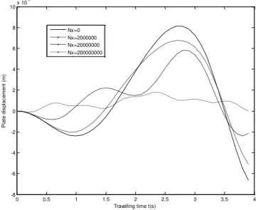
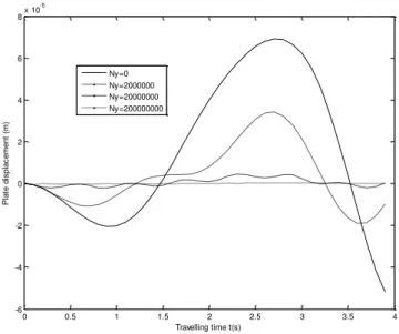
.Figures 1 and 2 depict the transverse displacement response of a simply supported isotropic rectangular plate under the action of concentrated forces moving at variable velocity for various values of axial force Nx and Ny respectively. These figures show that, for fixed values of subgrade
moduli K=40000 and Rotatory inertia correction factor Ro=50, as the values of Nx or Ny
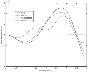
increas-es, the dynamic deflection of the isotropic rectangular plate decreases. Similar results are ob-tained when the simply supported plate is subjected to concentrated masses travelling at variable velocity as shown in figures 5 and 6. For various travelling time t, the deflection profile of the plate under the action of moving forces for various values of subgrade moduli K and for fixed values of axial forces Nx=2000000, Ny=20000 and Rotatory inertia correction factor Ro=50 are
shown in figure 3. It is observed that higher values of subgrade moduli K reduce the deflection profile of the vibrating plate structure. The same behaviour characterizes the deflection profile of the simply supported plate under the action of concentrated masses moving at variable velocity for various values of subgrade moduli K as shown in figure 7. Also, figures 4 and 8 display the displacement responses of the simply supported isotropic rectangular plate respectively to concen-trated forces and concenconcen-trated masses travelling with variable velocity for various values of rota-tory inertia Ro and for fixed values of axial forces Nx=20000 00, Ny=20000 and subgrade moduli
K=40000. These figures clearly show
Figure 1: Transverse displacement response of a simply supported isotropic rectangular plate under the actions
of concentrated forces travelling at variable velocities for various values of axial force along x direction Nx and
for fixed values of foundation constant K=40000, axial force along y Ny=20000 and rotatory inertia Ro=50.
0 0.5 1 1.5 2 2.5 3 3.5 4
-8 -6 -4 -2 0 2 4 6 8 10x 10
-5
Travelling time t(s)
P
la
te
d
is
p
la
c
e
m
e
n
t
(m
)
Latin A m erican Journal of Solids and Structures 12 (2015) 1296-1318 Figure 2: Transverse displacement response of a simply supported isotropic rectangular plate under the actions
of concentrated forces travelling at variable velocities for various values of axial force along y direction Ny and
for fixed values of foundation constant K=40000, axial force along x Nx=2000000 and rotatory inertia Ro=50.
Figure 3: Deflection profile of a simply supported isotropic rectangular plate under the actions of concentrated forces travelling at variable velocities for various values of foundation constant K
and for fixed values of axial force Nx=2000000, Ny=20000 and rotatory inertia Ro=50.
0 0.5 1 1.5 2 2.5 3 3.5 4
-6 -4 -2 0 2 4 6 8x 10
-5
Travelling time t(s)
P
la
te
d
is
p
la
c
e
m
e
n
t
(m
)
Ny=0 Ny=2000000 Ny=20000000 Ny=200000000
0 0.5 1 1.5 2 2.5 3 3.5 4
-1 -0.5 0 0.5 1 1.5
2x 10
-4
Travelling time t(s)
P
la
te
d
is
p
la
c
e
m
e
n
t
(m
)
Latin A m erican Journal of Solids and Structures 12 (2015) 1296-1318
Figure 4: Displacement response of a simply supported isotropic rectangular plate under the actions of concentrated forces travelling at variable velocities for various values of rotatory inertia Ro and
for fixed values of foundation constant K =40000, axial force Nx=2000000 and Ny=20000.
Figure 5: Transverse displacement response of a simply supported isotropic rectangular plate under
the actions of concentrated masses travelling at variable velocities for various values of axial force Nx
and for fixed values of foundation constant K =40000, Ny=20000 and rotatory inertia Ro=50
0 0.5 1 1.5 2 2.5 3 3.5 4
-2 -1 0 1 2 3 4 5 6 7x 10
-5
Travelling time t(s)
P
la
te
d
is
p
la
c
e
m
e
n
t
(m
)
Ro=550 Ro=1500 Ro=2500 Ro=15000
0 0.5 1 1.5 2 2.5 3 3.5 4
-6 -4 -2 0 2 4 6x 10
-4
Travelling time t(s)
P
la
te
d
is
p
la
c
e
m
e
n
t
(m
)
Latin A m erican Journal of Solids and Structures 12 (2015) 1296-1318 Figure 6: Transverse displacement response of a simply supported isotropic rectangular plate under the actions
of concentrated masses travelling at variable velocities for various values of axial force Ny and for fixed
values of foundation constant K =40000, Nx=2000000 and rotatory inertia Ro=50.
Figure 7: Deflection profile of a simply supported isotropic rectangular plate under the actions of concentrated masses travelling at variable velocities for various values of foundation constant K
and for fixed values of axial force Nx=2000000, Ny=20000 and rotatory inertia Ro=50.
0 0.5 1 1.5 2 2.5 3 3.5 4
-4 -3 -2 -1 0 1 2 3 4 5x 10
-4
Travelling time t(s)
P
la
te
d
is
p
la
c
e
m
e
n
t
(m
)
Ny=0 Ny=200000 Ny=2000000 Ny=20000000
0 0.5 1 1.5 2 2.5 3 3.5 4
-6 -4 -2 0 2 4 6 8x 10
-4
Travelling time t(s)
P
la
te
d
is
p
la
c
e
m
e
n
t
(m
)
Latin A m erican Journal of Solids and Structures 12 (2015) 1296-1318
Figure 8: Displacement response of a simply supported isotropic rectangular plate under the actions of concentrated masses travelling at variable velocities for various values of rotatory inertia Ro
and for fixed values of foundation constant K =40000, axial force Nx=2000000 and Ny=20000.
Figure 9: Response amplitudes of a simply supported isotropic rectangular plate under the actions of concentrated masses travelling at variable velocities for various values of the
mass ratio
0and for fixed values of of Nx=2000000, Ny=20000, K=40000 and Ro=50.0 0.5 1 1.5 2 2.5 3 3.5 4
-2 -1 0 1 2 3 4x 10
-3
Travelling time t(s)
P
la
te
d
is
p
la
c
e
m
e
n
t
(m
)
Ro=550 Ro=1500 Ro=2500 Ro=15000
0 0.5 1 1.5 2 2.5 3 3.5 4
-20 -10 0 10 20 30 40 50
Travelling time t(s)
P
la
te
d
is
p
la
c
e
m
e
n
t
(m
)
Latin A m erican Journal of Solids and Structures 12 (2015) 1296-1318 Figure 10: Comparison of the displacement response of moving force and moving
mass cases of a simply supported isotropic rectangular plate for fixed values
of Nx=2000000, Ny=20000, K=40000 and Ro=50.
that as the values of rotatory inertia correction factor increases, the displacement response of the simply supported plate under the action of both concentrated forces and concentrated masses travelling at variable velocity decreases. Also, for various travelling time t, the response ampli-tude of the isotropic plate under the action of accelerating traveling masses for fixed values of subgrade moduli K=40000, axial forces Nx=2000000, Ny=20000 and Rotatory inertia correction
factor Ro=50 are shown in figure 9. It is observed that larger values of the mass ratio,
0, in-creases the response amplitude of the isotropic plated subjected to accelerating masses.Finally, figure 10. depicts the comparison of the transverse displacement response of moving force and moving mass cases of a simply supported rectangular plate traversed by a moving load travelling at variable velocity for fixed values of Nx=2000000, Ny=20000, K=40000 and Ro=50.
Evidently, the response amplitude of the moving mass is higher than that of the moving force. This important result shows that, the moving force solution is not always an upper bound to the solution of the moving mass problem. Hence the inertia of the moving load must always be taken into consideration for accurate and reliable assessment of the response to moving load of elastic structures.
8 CONCLUSION
The problem of the flexural motions of a prestressed isotropic rectangular plate resting on elastic foundation and traversed by concentrated masses traveling with variable velocity has been inves-tigated. Closed form solution of the governing fourth order partial differential equations with variable and singular coefficients of the plate-mass problems is presented. For this two-dimensional dynamical problem, the solution techniques is based on the double Fourier finite sine
0 0.5 1 1.5 2 2.5 3 3.5 4
-4 -3 -2 -1 0 1 2 3 4 5x 10
-4
Travelling time t(s)
P
la
te
d
is
p
la
c
e
m
e
n
t
(m
)