Flexural motions under accelerating loads of structurally
pre-stressed beams with general boundary conditions
Abstract
The transverse vibration of a prismatic Rayleigh beam rest-ing on elastic foundation and continuously acted upon by concentrated masses moving with arbitrarily prescribed ve-locity is studied. A procedure involving generalized finite integral transform, the use of the expression of the Dirac delta function in series form, a modification of the Struble’s asymptotic method and the use of the Fresnel sine and cosine functions is developed to treat this dynamical beam prob-lem and analytical solutions for both the moving force and moving mass model which is valid for all variant of classical boundary conditions are obtained. The proposed analyti-cal procedure is illustrated by examples of some practianalyti-cal engineering interest in which the effects of some important parameters such as boundary conditions, prestressed func-tion, slenderness ratio, mass ratio and elastic foundation are investigated in depth. Resonance phenomenon of the vibrat-ing system is carefully investigated and the condition under which this may occur is clearly scrutinized. The results pre-sented in this paper will form basis for a further research work in this field.
Keywords
Rayleigh beam, resonance phenomenon, asymptotic method, concentrated masses, transverse vibration, slenderness ratio.
S. T. Oni and B. Omolofe∗
Department of Mathematical Sciences, School of Sciences, Federal University of Technology, PMB 704, Akure, Ondo state – Nigeria
Received 21 Mar 2010; In revised form 21 Jun 2010
∗Author email:
babatope [email protected]
1 INTRODUCTION
publications dealt with a beam model whose dynamic characteristics are described by Euler-Bernoulli beam equations. It is however well known that if the slenderness ratio is large, or vibration of higher modes is concerned, the use of classical Bernoulli-Euler beam theory can-not ensure sufficient accuracy. Thus, a beam theory which takes into account the effects of shearing deformation or rotatory inertia or both must be adopted for more accurate analysis [10].
Even with the inclusion of shear deformation and rotatory inertia into the equation of motion, a good number of these studies have considered a much simpler problem where the motion of the moving mass is described by a constant velocity type of motion. However, situation arises when the moving mass accelerates by a forward force or decelerates, reduces speed and come to rest at any desired position on the beam and causing the friction between the mass and the beam to increase considerably. Under such condition, the vibrating system exhibits dynamic behaviour which may be more complicated.
Previous studies where such a dynamical system was investigated are Wang [20] who studied the dynamical analysis of a finite inextensible beam with an attached accelerating mass. He employed the Galerkin procedure in conjunction with the method of numerical integration to tackle the partial differential equations which describe the transient vibrations of the beam-mass system. He concluded that the applied forward force amplifies the speed of the beam-mass and the displacement of the beam. Though the theory developed here is versatile, its application is only limited to the case of beams executing flexural motions according to the simple Bernoulli-Euler theory of flexure. Nevertheless, it is easy to see that a typical element of an elastic system performs not only a translatory motion but also rotates [18]. Hilal and Ziddeh [6] investigated the vibration analysis of beams with general boundary conditions traversed by a single point force traveling with variable velocity. They obtained analytical solution to the beam problem and compared the results with same beam under the actions of a concentrated force traveling at constant velocity. Their method of solution is only suitable to handle an approximate model in which the vehicle-structure interaction is completely neglected; this type of beam model has been described by Guiseppe and Alessandro [13] as the crudest approximation known to the literature of assessing the dynamic response of an elastic system which supports moving concentrated masses. Lee [9] tackled the transverse vibration of a Timoshenko beam acted on by an accelerating mass. In his study, he presented numerical results for a prescribed constant acceleration or deceleration and the slenderness ratio of the beam. He figured-out that the separation of the mass from the beam may occur for a Timoshenko beam when the traveling speed of the mass is large due to large initial traveling speed or large prescribed acceleration. Nevertheless, his method of solution is incapable of handling moving load problems involving end conditions other than simple ones.
2 THEORETICAL FORMULATION
Consider the flexural motion of a uniform finite Rayleigh beam resting on an elastic foundation and carrying a relatively large massM. The mass M is assumed to touch the beam at timet = 0 and travel across it with a non-uniform velocity such that the motion of the contact point of the moving load is described by the function
f(t)=x0+ct+
1 2at
2
(1)
where x0 is the point of application of force P = M g at the instance t = 0, c is the initial
velocity andais the constant acceleration of motion. Furthermore, the beam’s properties such as moment of inertiaI, and the mass per unit lengthµof the beam do not vary along the span L of the beam.
The equation of motion with damping neglected is given by the fourth order partial differ-ential equation
EI∂ 4
V(x,t)
∂x4 −N
∂2V(x,t)
∂x2 +µ
∂2V(x,t)
∂ t2 −µR0∂
4 V(x,t)
∂x2∂ t2 +KV(x, t)
+M δ[x−(x0+ct+ 1 2at
2
)] [∂2V(x,t)
∂ t2 +2(c+at)
∂2V(x,t)
∂x∂ t +(c+at)
2∂2V(x,t)
∂x2 +a ∂V(x,t)
∂x ]
=M gδ[x−(x0+ct+ 1 2at
2 )]
(2)
wherex is the spacial coordinate, tis the time,V (x, t)is the Transverse Displacement, EI is the flexural rigidity of the structure,µ is the mass per unit length of the beam,N is the axial force, R0 is the rotatory inertia factor, K is the elastic foundation stiffness, M is the mass
of the traversing concentrated load, g is the acceleration due to gravity and δ(⋅) is the well known Dirac delta function.
The boundary conditions of the structure under consideration is arbitrary and the initial conditions without any loss of generality is taken as
V(x,0)=0,∂V(x,0)
∂t =0∀x (3)
Since the load is assumed to be of mass M and the time t is assumed to be limited to that interval of time within which the mass is on the beam, that is
0≤f(t)≤L (4)
3 ANALYTICAL PROCEDURES
Fourier cosine series and then reducing the modified form of the fourth order partial differential equation above using the generalized finite integral transform. The resulting transformed differential equation having some variable coefficients is then simplified using the modified Struble’s asymptotic technique.
3.1 The generalized finite integral transform
For the dynamical systems, the governing equation is a fourth order partial differential equation with variable and singular coefficients. The Generalized Finite Integral Transform (GFIT) is employed to remove the singularities in the governing equations and to reduce it to a sequence of second order ordinary differential equations with variable coefficients. This generalized finite integral transform is defined by
V(m, t)=∫ L
0
V(x, t)Um(x)dx (5)
with the inverse
V(x, t)=
∞ ∑
m=1
µ Vm
V(m, t)Um(x) (6)
where
Vm=∫ L
0
µUm2(x)dx (7)
and Um(x) is any function chosen such that the pertinent boundary conditions are satisfied. An appropriate selection of functions for beam problems are beam mode shapes. Thus, the mth normal mode of vibration of a uniform beam
Um(x)=sin λmx
L +Amcos λmx
L +Bmsinh λmx
L +Cmcosh λmx
L (8)
is chosen as a suitable kernel of the integral transform (5) where,λmis the mode frequency,Am, Bm,Cm are constants which are obtained by substituting (8) into the appropriate boundary conditions.
3.2 Operational simplification
By applying the generalized finite integral transform (5), equation (2) can be written as
H1θ(0, L, t)+H1θA(t)−H2θB(t)+Vtt(m, t)−R0θC(t)+H3V(m, t)+θD(t)+θE(t)+θF(t)+θG(t) =M g
µ Um(x0+ct+
1 2at
2)
(9) where
H1=
EI µ , H2=
N µ, H3=
K
θ(0, L, t)=[∂
3
V(x, t)
∂x3 Um(x)−
∂2
V(x, t) ∂x2
dUm(x) dx +
∂V(x, t) ∂x
d2
Um(x)
dx2 −V(x, t)
d3
Um(x) dx3 ]L0
(11)
θA(t)=∫ L
0
V(x, t)d
4
Um(x)
dx4 dx (12a)
θB(t)=∫ L
0
∂2
V(x, t)
∂x2 Um(x)dx (12b)
θC(t)=∫ L
0
∂4
V(x, t)
∂x2∂t2 Um(x)dx (12c)
θD(t)=∫ L
0
M
µ δ[x−(x0+ct+ 1 2at
2
)]∂2V∂t(x, t2 )Um(x)dx (12d)
θE(t)=∫ L
0
2M(c+at)
µ δ[x−(x0+ct+ 1 2at
2
)]∂2V(x, t)
∂x∂t Um(x)dx (12e)
θF(t)=∫ L
0
M(c+at)2
µ δ[x−(x0+ct+ 1 2at
2
)]∂2V(x, t)
∂x2 Um(x)dx, and (12f)
θG(t)=∫ L
0
aM
µ δ[x−(x0+ct+ 1 2at
2
)]∂V∂x(x, t)Um(x)dx (12g)
In order to evaluate the integrals (12a-12g), use is made of the property of the Dirac Delta function as an even function to express it in Fourier cosine series namely:
δ[x−(x0+ct+
1 2at
2 )]= 1
L+ 2 L
∞ ∑
n=1
cosnπ
L (x0+ct+ 1 2at
2
)cosnπx
L (13)
Vtt(m, t)+[ω
2
n+ K
µ]V(m, t)−R0
∞ ∑
k=1
Vtt(k, t)Ha(k, m)− N
µ
∞ ∑
k=1
V(k, t)Ha(k, m)
+ε∗{
∞ ∑
k=1
Vtt(k, t)Hb(k, m)+2
∞ ∑
n=1 ∞ ∑
k=1
Vtt(k, t)Hc(k, m, n)cos nπ
L (x0+ct+ 1 2at
2 )
+2(c+at)
∞ ∑
k=1
Vt(k, t)Hd(k, m)+4(c+at)
∞ ∑
n=1 ∞ ∑
k=1
Vt(k, t)He(k, m, n)cos nπ
L (x0+ct+ 1 2at
2 )
+(c+at)2
∞ ∑
k=1
V(k, t)Hf(k, m)+2(c+at)2
∞ ∑
n=1 ∞ ∑
k=1
V(k, t)Hg(k, m, n)cosnπ
L (x0+ct+ 1 2at 2 ) +a ∞ ∑
k=1
V(k, t)Hi(k, m)+2a
∞ ∑
n=1 ∞ ∑
k=1
V(k, t)Hj(k, m, n)cos nπ
L (x0+ct+ 1 2at
2 )}=
M g µ [sin
λm
L (x0+ct+ 1 2at
2
)+Amcos λm
L (x0+ct+ 1 2at
2
)+Bmsinh λm
L (x0+ct+ 1 2at
2 )+
Cmcosh λm
L (x0+ct+ 1 2at 2 )] (14) where
Ha(k, m)= 1 τk(x)∫
L
0
Uk′′(x)Um(x)dx (15a)
Hb(k, m)= 1 τk(x)∫
L
0
Uk(x)Um(x)dx (15b)
Hc(k, m, n)= 1 τk(x)∫
L
0
Uk(x)Um(x)cos nπx
L dx (15c)
Hd(k, m)= 1 τk(x)∫
L
0
Uk′(x)Um(x)dx (15d)
He(k, m, n)= 1 τk(x)∫
L
0
Uk′(x)Um(x)cos nπx
L dx (15e)
Hf(k, m)= 1 τk(x)∫
L
0
Uk′′(x)Um(x)dx (15f)
Hg(k, m, n)= 1 τk(x)∫
L
0
Uk′′(x)Um(x)cos nπx
L dx (15g)
Hi(k, m)= 1 τk(x)∫
L
0
Uk′(x)Um(x)dx (15h)
Hj(k, m, n)= 1 τk(x)∫
L
0
Uk′(x)Um(x)cos nπx
ω2n=λ
4
m L4
EI
µ (15j)
ε∗= M
µ L (15k)
Equation (14) is the transformed equation governing the problem of a uniform Bernoulli-Euler beam on a constant elastic foundation. This coupled non-homogeneous Second order ordinary differential equation holds for all variants of the classical boundary conditions.
In what follows, two special cases of equation (14) are considered
3.3 Solution of the transformed governing equation
Case I: The Moving Force Problem. The differential equation describing the behaviour of a Rayleigh beam on an elastic foundation to a moving force moving at variable velocity may be obtained from equation (14) by setting ε∗=0. It is an approximate model, which assumes the inertia effect of the moving mass negligible and only the force effect of the moving load is taken into consideration, thus in this case one obtains
Vtt(m, t)+[ω
2
n+ K
µ]V(m, t)−R0
∞ ∑
k=1
Vtt(k, t)Ha(k, m)− N
µ
∞ ∑
k=1
V(k, t)Ha(k, m)=
M g µ [sin
λm
L (x0+ct+ 1 2at
2
)+Amcos λm
L (x0+ct+ 1 2at
2
)+Bmsinh λm
L (x0+ct+ 1 2at
2 )+
Cmcosh λm
L (x0+ct+ 1 2at
2 )]
(16)
Evidently, an exact analytical solution to equation (16) is not possible. Though the equa-tion may readily yield to numerical technique, an analytical approximate method is desirable as solutions so obtained often shed light on vital information about the vibrating system. Thus, we are going to use a modification of the asymptotic method due to Struble’s extensively discussed in [14]. To this effect, equation (16) is rearranged to take the form
Vtt(m, t) +
γ2
nf
[1−ε0LHa(m, m)]
V(m, t) − ε0
[1−ε0LHa(m, m)]
⎡⎢ ⎢⎢ ⎢⎢ ⎢⎢ ⎢⎢ ⎣
∞ ∑
k=1
k≠m
LHa(k, m)Vtt(k, t) +N0
∞ ∑
k=1
k≠m
Ha(k, m)V(k, m)
⎤⎥ ⎥⎥ ⎥⎥ ⎥⎥ ⎥⎥ ⎦
= M g
µ[1−ε0LHa(m, m)][
sinλm
L (x0+ct+
1 2at
2
) +Amcos
λm
L (x0+ct+
1 2at
2
) +Bmsinh
λm
L (x0+ct+
1 2at
2
)
+Cmcosh
λm
L (x0+ct+
1 2at
2)]
(17)
ε0=
R0
L , N0= LN R0µ, γ
2
nf =ω
2
nk−N0Ha(m, m), ω
2
nk=ω
2
n+ K
µ and Ha(m, m)=Ha(k, m) ∣k=m
(18) By this technique, one seeks the modified frequency corresponding to the frequency of the free system due to the presence of the effect of the rotatory inertia. An equivalent free system operator defined by the modified frequency then replaces equation (17). Thus, we set the right-hand-side of (17) to zero and consider a parameter η0 < 1 for any arbitrary ratio ε0,
defined as
η0=
ε0
1+ε0
(19)
so that
ε0=η0+O(η 2
0) (20)
Substituting equation (20) into the homogeneous part of equation (17) one obtains
Vtt(m, t) +γnf2 (1+η0LHa(m, m))V(m, t)−
η0(1+η0LHa(m, m))
⎡⎢ ⎢⎢ ⎢⎢ ⎢⎢ ⎢⎢ ⎣
∞ ∑
k=1
k≠m
LHa(k, m)Vtt(k, t) +N0
∞ ∑
k=1
k≠m
Ha(k, m)V(k, m)
⎤⎥ ⎥⎥ ⎥⎥ ⎥⎥ ⎥⎥ ⎦
=0 (21)
When η is set to zero in equation (17) a situation corresponding to the case in which the rotatory inertia effect is regarded as negligible is obtained, then the solution of equation (17) can be written as
Vnf(m, t)=Cnfcos[ωnft−ψnf] (22) where Cnf,ωnf and ψnf are constants.
Furthermore as η0 < 1 Struble’s technique requires that the asymptotic solutions of the
homogeneous part of the equation (17) be of the form
V(m, t)=Λ(m, t)cos[ωnft−φ(m, t)]+η0V¯(1, t)+O(η 2
0) (23)
where Λ(m, t)and φ(m, t) are slowly varying functions of time.
To obtain the modified frequency, equation (23) and its derivatives are substituted into equation (21) and neglecting terms which do not contribute to variational equations, one obtains.
2Λ(m, t)γnfφ˙(m, t)cos[γnft−φ(m, t)]−2 ˙Λ(m, t)γnfsin[γnft−φ(m, t)]
−η0γ 2
nfLHa(m, m)Λ(m, t)cos[γnft−φ(m, t)]=0
retaining terms toO(η0) only.
The variational equations are obtained by equating the coefficients of sin[γnft−φ(m, t)] and cos[γnft−φ(m, t)]on both sides of the equation (24). Thus,
−2 ˙Λ(m, t)γnf =0 (25) and
2Λ(m, t)γnfφ˙(m, t)−η0γ 2
nfLHa(m, m)Λ(m, t)=0 (26)
Solving equations (25) and (26) respectively gives
Λ(m, t)=Cmf (27)
and
φ(m, t)=−η0LγnfHa(m, m) 2ωnf
t+ψmf (28)
where C0
mf and ψmf are constants.
Therefore, when the effect of the rotatory inertia is considered, the first approximation to the homogeneous system is
V(m, t)=Cmf0 Cos[γmft−ψmf] (29) where
γmf = γnf
2 [2+η0LHa(m, m)] (30)
represents the modified natural frequency due to the effect of the rotatory inertia R0. It is
observed that when η0= 0, we recover the frequency of the moving force problem when the
rotatory inertia effect of the beam is neglected. Thus, to solve the non-homogeneous equation (17), the differential operator which acts onV(m, t) and V(k, t) is replaced by the equivalent free System operator defined by the modified frequency γmf, thus using equation (30) the homogeneous part of equation (17) can be written as
d2
V(m, t) dt2 +γ
2
mfV(m, t)=0 (31)
Hence, the entire equation (17) takes the form
d2
V(m, t) dt2 +γ
2
mfV(m, t)=P
0
mf[sin λm
L (x0+ct+ 1 2at
2
)+Amcos λm
L (x0+ct+ 1 2at
2 )
+Bmsinh λm
L (x0+ct+ 1 2at
2
)+Cmcosh λm
L (x0+ct+ 1 2at
2 )]
where
Pmf0 = M g
µ[1−η0LHa(m, m)]
(33)
Solving equation (32) in conjunction with the initial conditions gives expression for ¯V(m, t)which on inversion yields
V(x, t)= 1 τ∗(x)
∞ ∑
m=1
⎛ ⎝
P0
mfsinγmft
γmf (
D13S[q12+q10t] −D14C[q12+q10t] −D11S[q11+q10t] +D12C[q11+q10t]
+D23C[q11+q10t] +D24S[q11+q10t] −D21C[q12+q10t] −D22S[q12+q10t] +E14erf i[q22+q20t]
−E13erf[q22+q20t] +E12erf i[q21+q20t] −E11erf[q21+q20t] +E24erf[q22+q20t] +E23erf i[q22+q20t]
+E22erf[q21+q20t] + −E21erf i[q21+q20t] −C 0 2) −
P0
mfcosγmft
γmf (
D11C[q11+q10t] +D12S[q11+q10t]
−D13C[q12+q10t] −D14S[q12+q10t] +D21S[q12+q10t] −D22C[q12+q10t] −D23S[q11+q10t]
−D24S[q11+q10t] +iE11erf[q21+q20t] +iE12erf i[q21+q20t] +iE13erf[q22+q20t]
+iE14erf i[q22+q20t] +iE21erf i[q21+q20t] −iE22erf[q21+q20t] −iE23erf i[q22+q20t]
+iE24erf[q22+q20t] +C 0 1)) (sin
λmx
L +Amcos λmx
L +Bmsinh λmx
L +Cmcosh λmx
L )
(34)
where C(x) and S(x)are the well known time-dependent Fresnel integrals defined by
C(x)=∫ x
0 cos
πt2
2 dt and S(x)=∫ x
0 sin
πt2
2 dt and
D11=
1 2√a0
√π
2Cos( b21
4a0 −
c0), D12=
1 2√a0
√π
2Sin( b21
4a0−
c0)
D13=
1 2√a0
√π
2Cos( b2
2
4a0 −
c0), D14=
1 2√a0
√π
2Sin( b2
2
4a0−
c0)
D21=
Am 2√a0
√π
2Cos( b2
2
4a0 −
c0), D22=
Am 2√a0
√π
2Sin( b2
2
4a0−
c0)
D23=
Am 2√a0
√π
2Cos( b21
4a0 −
c0), D24=
Am 2√a0
√π
2Sin( b21
4a0−
c0)
E11=
Bm√π 8√a0
e−
b23 4a0−c0e
b23
2a0, E12= Bm
√π
8√a0
e−
b23
4a0−c0e2c0, E13= Bm
√π
8√a0
e−
b24 4a0−c0e
b24 2a0
E14=
Bm√π 8√a0
e−
b24
4a0−c0e2c0, E21= Cm
√
π 8√a0
e−
b23
4a0−c0e2c0, E22=Cm
√
π 8√a0
e−
b23 4a0−c0e
E23=
Cm√π 8√a0
e−
b24
4a0−c0e2c0, E24= Cm
√π
8√a0
e−
b24 4a0−c0e
b24 2a0
q10=
2a0 √
2πa0
, q11=
b1 √
2πa0
, q12=
b2 √
2πa0
, q20=
2a0
2√a0
, q21=
b3
2√a0
, q22=
b4
2√a0
a0=
λma 2L , b1=
cλm
L −γmf, b2= cλm
L +γmf, b3= cλm
L −iγmf, b3= cλm
L +iγmf
C10=D11C(q11) +D12S(q11) −D13C(q12) −D14S(q12) +D21S(q12) −D22C(q12) −D23S(q11) −D24C(q11)
+iE11erf(q12) +iE12erf i(q21) +iE13erf(q22) +iE14erf i(q22) +iE21erf i(q21) −iE22erf(q21) −iE23erf i(q22)
+iE24erf(q22)
C20=D13S(q12) −D14C(q12) −D11S(q11) +D12C(q11) +D23C(q11) +D24S(q11) −D21C(q12) −D22S(q12)
+E14erf i(q22) −E13erf(q22) +E12erf i(q22) −E11erf(q21) +E24erf(q22) +E23erf i(q22) +E22erf(q21)
+E21erf i(q21)
i=√−1
and
τ∗(x)=∫ L
0
Um2(x)dx (35)
Equation (34) represents the transverse displacement response to forces moving with non-uniform velocities of prestressed non-uniform Rayleigh beam resting on elastic foundation and having arbitrary end support conditions.
Vtt(m, t) +γmf2 V(m, t) +ε∗{
∞ ∑
k=1
Vtt(k, t)Hb(k, m) +2
∞ ∑
n=1
∞ ∑
k=1
Vtt(k, t)Hc(k, m, n)cos
nπ
L (x0+ct+
1 2at
2
)
+2(c+at)
∞ ∑
k=1
Vt(k, t)Hd(k, m) +4(c+at)
∞ ∑
n=1
∞ ∑
k=1
Vt(k, t)He(k, m, n)cos
nπ
L (x0+ct+
1 2at
2)
+(c+at)2
∞ ∑
k=1
V(k, t)Hf(k, m) +2(c+at)
2 ∞
∑
n=1
∞ ∑
k=1
V(k, t)Hg(k, m, n)cos
nπ
L (x0+ct+
1 2at 2 ) +a ∞ ∑
k=1
V(k, t)Hi(k, m) +2a
∞ ∑
n=1
∞ ∑
k=1
V(k, t)Hj(k, m, n)cos
nπ
L (x0+ct+
1 2at
2
)}=M g
µ [sin λm
L (x0+ct+
1 2at
2
)
+Amcos
λm
L (x0+ct+
1 2at
2) + Bmsinh
λm
L (x0+ct+
1 2at
2) +
Cmcosh
λm
L (x0+ct+
1 2at
2) ]
(36)
As in the previous case, an exact analytical solution to the above equation is not possible. The same technique used in case I is employed to obtain the modified frequency due to the presence of the moving mass, namely
γmm=γmf⎧⎪⎪⎨⎪⎪
⎩1−
η∗ 2
⎡⎢ ⎢⎢
⎣Hb(m, m)−
(c2Hf(m, m)+aHi(m, m)) γ2 mf ⎤⎥ ⎥⎥ ⎦ ⎫⎪⎪ ⎬⎪⎪ ⎭ (37) where
η∗= ε
∗
1+ε∗ and ε ∗= M
µ L, Hb(m, m)=Hb(k, m)∣k=m
,
Hf(m, m)=Hf(k, m)∣ k=m
Hi(m, m)=Hi(k, m)∣ k=m
(38)
retaining O(λ) only.
Thus, equation (36) takes the form
d2
V(m, t) dt2 +γ
2
mmV(m, t)=η∗Lg[sin λm
L (x0+ct+ 1 2at
2
)+Amcos λm
L (x0+ct+ 1 2at
2 )
+Bmsinh λm
L (x0+ct+ 1 2at
2
)+Cmcosh λm
L (x0+ct+ 1 2at
2 )]
(39)
This is analogous to equation (32). Thus, using similar argument as in case I, V(m, t)can be obtained and which on inversion yields
V(x, t)= 1 τ∗(x)
∞ ∑
m=1 η∗Lg
γmm(sin
γmmt(D13S[q12+q10t] −D14C[q12+q10t] −D11S[q11+q10t] +D12C[q11+q10t]
+D23C[q11+q10t] +D24S[q11+q10t] −D21C[q12+q10t] −D22S[q12+q10t] +E14erf i[q22+q20t]
−E13erf[q22+q20t] +E12erf i[q21+q20t] −E11erf[q21+q20t] +E24erf[q22+q20t] +E23erf i[q22+q20t]
+E22erf[q21+q20t] + −E21erf i[q21+q20t] −C 0
2) −cosγmmt(D11C[q11+q10t] +D12S[q11+q10t]
−D13C[q12+q10t] −D14S[q12+q10t] +D21S[q12+q10t] −D22C[q12+q10t] −D23S[q11+q10t]
−D24S[q11+q10t] +iE11erf[q21+q20t] +iE12erf i[q21+q20t] +iE13erf[q22+q20t]
+iE14erf i[q22+q20t] +iE21erf i[q21+q20t] −iE22erf[q21+q20t] −iE23erf i[q22+q20t]
+iE24erf[q22+q20t] +C01) ) (sin λmx
L +Amcos λmx
L +Bmsinh λmx
L +Cmcosh λmx
L )
where all parameters are as previously defined, butγmm has replacedγmf
Equation (40) represents the transverse displacement response to concentrated masses, moving with non-uniform velocity of highly prestressed uniform Rayleigh beam resting on elastic foundation. Equation (40) is valid for all variants of classical boundary conditions.
4 APPLICATIONS
In this section, the forgoing analyses are illustrated by various practical examples. Specifically, classical boundary conditions such as simply supported boundary conditions, clamped-clamped end conditions and clamped-free end conditions are considered.
4.1 Simply Supported Boundary Conditions
In this case, the displacement and the bending moment vanish. Thus
V(0, t)=0=V(L, t), ∂
2
V(0, t) ∂x2 =0=
∂2V(L, t)
∂x2 (41)
Hence for normal modes
Um(0)=0=Um(L),
∂2Um(0) ∂x2 =0=
∂2Um(L)
∂x2 (42)
which implies that
Uk(0)=0=Uk(L),
∂2
Uk(0) ∂x2 =0=
∂2
Uk(L)
∂x2 (43)
Applying (41) and (42), one obtains
Am=Ak =0; Bm=Bk=0; Cm=Ck=0
λm=mπ and λk=kπ (44)
Thus, the moving force problem is reduced to a non-homogeneous second order ordinary differential equation
d2
V(m, t) dt2 +α
2
mfV(m, t)= Pmf
µ sin(x0+ct+ 1 2at
2
) (45)
where
α2mf =
EI(mπL )4+Kµ +Nµ (mπL )2 1+R0(mπL )
2 and Pmf =
M g
1+R0(mπL )
2 (46)
V(x, t)= 2
L ∞ ∑
m=1
Pmf√π 2µαmf√2a0(
sinαmft[cos( b2
2
4a0 −
c0)S(
b2+2a0t
√
2πa0 )−
C(b√2+2a0t 2πa0 )
sin( b
2 2
4a0 −
c0)
+cos( b
2 1
4a0−
c0)S(
b1+2a0t
√
2πa0 )−
C(b1√+2a0t 2πa0 )
sin( b
2 1
4a0−
c0)−cos(
b2 2
4a0 −
c0)S(
b2
√
2πa0)
+C(√b2 2πa0)
sin( b
2 2
4a0 −
c0)−cos(
b2 1
4a0−
c0)S(
b1
√
2πa0)+
C(√b1 2πa0)
sin( b
2 1
4a0−
c0)]
−cosαmft[cos( b2
1
4a0−
c0)C(
b1+2a0t
√
2πa0 )+
S(b√1+2a0t 2πa0 )
sin( b
2 1
4a0 −
c0)−
cos( b
2 2
4a0−
c0)C(
b2+2a0t
√
2πa0 )−
S(b2√+2a0t 2πa0 )
sin( b
2 2
4a0−
c0)−cos(
b2 1
4a0 −
c0)C(
b1
√
2πa0)−
S(√b1 2πa0)
sin( b
2 1
4a0−
c0)
+cos( b
2 2
4a0−
c0)C(
b2
√
2πa0)+
S(√b2 2πa0)
sin( b
2 2
4a0 −
c0)]) (sin
mπ L x)
(47)
which represents the transverse displacement response to forces moving with non-uniform velocity of a simply supported uniform Rayleigh beam resting on elastic foundation.
Following arguments similar to those in the last sections, use is made of the modified asymptotic method due to Struble to obtain the modified natural frequency due to the presence of inertia terms for the simply supported beam given as
αmm=αmf⎧⎪⎪⎨⎪⎪
⎩1−
η 2
⎡⎢ ⎢⎢ ⎣2+
(2c2
R(m, m)−R2(m, m, n))
α2 mf ⎤⎥ ⎥⎥ ⎦ ⎫⎪⎪ ⎬⎪⎪ ⎭ (48) where
R(m, m)=(mπ L )
2
and R2(m, m, n)= ∞ ∑
n=1
8am2
L(4m2−n2)cos
nπ
L (x0+ct+ 1 2at
2
) (49)
neglecting higher order terms of λ. Thus, the simply supported moving mass problem reduces to
d2
V(m, t) dt2 +α
2
mmV(m, t)=ηLgsin mπ
L (x0+ct+ 1 2at
2
) (50)
V(x, t)= 2
L ∞ ∑
m=1
ηLg√π 2µαmm√2a0(
sinαmmt[Cos( b2
2
4a0 −
c0)S(
b2+2a0t
√
2πa0 )−
C(b√2+2a0t 2πa0 )
sin( b
2 2
4a0 −
c0)
+cos( b
2 1
4a0−
c0)S(
b1+2a0t
√
2πa0 )−
C(b√1+2a0t 2πa0 )
sin( b
2 1
4a0−
c0)−cos(
b2 2
4a0 −
c0)S(
b2
√
2πa0)
+C(√b2 2πa0)
sin( b
2 2
4a0−
c0)−cos(
b2 1
4a0−
c0)S(
b1
√
2πa0)+
C(√b1 2πa0)
sin( b
2 1
4a0−
c0)]
−cosαmmt[cos( b2
1
4a0−
c0)C(
b1+2a0t
√
2πa0 )+
S(b1√+2a0t 2πa0 )
sin( b
2 1
4a0−
c0)−
cos( b
2 2
4a0 −
c0)C(
b2+2a0t
√
2πa0 )−
S(b√2+2a0t 2πa0 )
sin( b
2 2
4a0−
c0)−cos(
b2 1
4a0 −
c0)C(
b1
√
2πa0)−
S(√b1 2πa0)
sin( b
2 1
4a0 −
c0)+ cos(
b2 2
4a0−
c0)C(
b2
√
2πa0)+
S(√b2 2πa0)
sin( b
2 2
4a0−
c0)]) (sin
mπ L x)
(51)
This represents the transverse-displacement response to a concentrated mass moving with non-uniform velocity of a simply supported uniform Rayleigh beam resting on elastic founda-tion.
5 COMMENTS ON CLOSED FORM SOLUTIONS
It is pertinent at this juncture to establish conditions under which resonance occurs. This phenomenon in structural and highway engineering is of great concern to researchers or in particular, design engineers, because, for example, it causes cracks, permanent deformation and destruction in structures. Bridges and other structures are known to have collapsed as a result of resonance occurring between the structure and some signals traversing them.
Equation (47) clearly shows that the Simply Supported elastic beam resting on elastic foundation and traversed by moving force reaches a state of resonance whenever
αmf = mπcc
L , αmf = mπcc
L +2a0tc (52)
while equation (51) indicates that the same beam under the action of moving mass will expe-rience resonance effect whenever
αmm= mπcc
L , αmm = mπcc
L +2a0tc (53)
whereccandtcare respectively the critical velocity and critical time at which resonance occurs. From equation (48), we know that
αmm=αmf⎧⎪⎪⎨⎪⎪
⎩1−
η 2
⎡⎢ ⎢⎢ ⎣2+
(2c2
R(m, m)−R2(m, m, n))
which implies
αmf =
mπcc L
{1−η2[2+
(2c2R(m,m)−R2(m,m,n)) α2
mf ]}
(55)
It is therefore evident, that for the same natural frequency, the critical velocity for the system consisting of a Simply Supported Elastic Beam resting on an elastic foundation and traversed by concentrated forces moving with a non-uniform speed is greater than that of the moving mass problem. Thus, for the same natural frequency of an elastic beam, resonance is reached earlier in the moving mass system than in the moving force system.
For the resonance conditions for other classical boundary conditions, equation (34) clearly shows that the uniform elastic beam resting on an elastic foundation and traversed by concen-trated forces moving with variable velocities reaches a state of resonance whenever
γmf = λmcc
L and γmf = λmcc
L + 2a0t
L (56)
while equation (40) shows that the same beam under the action of a moving mass experiences resonance effect whenever
γmm= λmcc
L and γmm= λmcc
L + 2a0t
L (57)
From equation (37)
γmm=γmf⎧⎪⎪⎨⎪⎪
⎩1−
η∗ 2
⎡⎢ ⎢⎢
⎣(Hb(m, m))−
c2(
Hf(m, m)+aHi(m, m)) γ2
mf
⎤⎥ ⎥⎥ ⎦ ⎫⎪⎪ ⎬⎪⎪
⎭ (58)
which implies
γmf =
λmcc L
1−η∗
2 [(Hb(m, m))−
c2(H
f(m,m)+aHi(m,m)) γ2
mf ]
(59)
Evidently, from equation (58) and (59), the same results and analysis obtained in the case of a Simply Supported Bernoulli-Euler beam are obtained for all other examples of classical boundary conditions.
6 NUMERICAL RESULTS AND DISCUSSION
We shall illustrate the analysis proposed in this paper by considering a homogenous beam of modulus of elasticity E = 3.1×10¹⁰N/m2, the moment of inertiaI =2.87698×10⁻³m4,
the beam span L = 150m and the mass per unit length of the beam µ=2758.291 Kg/m. The values of foundation moduli are varied between 0N/m3
and 400000N/m3
, the values of axial force N is varied between 0 N and 2⋅0×108
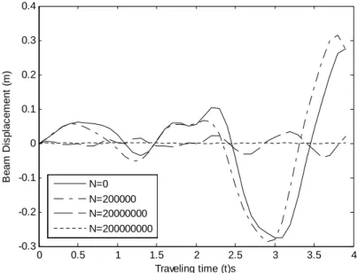
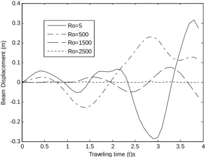
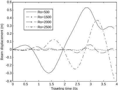
Figure 1 displays the transverse displacement response of a clamped-clamped uniform Rayleigh beam under the action of concentrated forces moving at variable velocity for various values of axial force N and for fixed values of foundation modulus K=40000 and Rotatory inertia correction factor Ro=50. The figure shows that as N increases, the dynamic deflec-tion of the uniform beam decreases. Similar results are obtained when the fixed-fixed beam is subjected to a concentrated masses traveling at variable velocity as shown in figure 4. For various traveling timet, the deflection profile of the beam for various values of foundation mod-ulus K and for fixed values of axial force N=200000 and Rotatory inertia correction factor Ro=50 are shown in figure 2. It is observed that higher values of foundation modulus reduce the deflection profile of the vibrating beam. The same behaviour characterizes the deflection profile of the clamped-clamped beam under the action of concentrated masses moving at vari-able velocity for various values of foundation modulus K as shown in figure 5. Also, figures 3 and 6 display the response amplitudes of the clamped-clamped uniform Rayleigh beam re-spectively to concentrated forces and masses traveling at variable velocity for various values of rotatory inertia Ro and for fixed values of axial force N=200000 and foundation modulus K=40000. These figures clearly show that as the values of rotatory inertia correction factor
increases, the response amplitudes of the clamped-clamped uniform beam under the action of both concentrated forces and masses traveling at variable velocity decrease. Figure 7 depicts the comparison of the transverse displacement response of moving force and moving mass cases of a clamped-clamped uniform Rayleigh bean traversed by a moving load traveling at variable velocity for fixed values ofN=200000,K=400000 andRo=50.
values of rotatory inertia Ro and for fixed values of axial force N=200000 and foundation
modulusK=40000.
0 0.5 1 1.5 2 2.5 3 3.5 4
-0.3 -0.2 -0.1 0 0.1 0.2 0.3 0.4
Traveling time (t)s
B
e
a
m
D
is
p
la
c
e
m
e
n
t
(m
)
N=0 N=200000 N=20000000 N=200000000
0 0.5 1 1.5 2 2.5 3 3.5 4 -0.8
-0.6 -0.4 -0.2 0 0.2 0.4 0.6
Traveling time (t)s
B
e
a
m
D
is
p
la
c
e
m
e
n
t
(m
)
K=0 K=4000 K=40000 K=400000
Figure 2 Deflection profile of a clamped-clamped uniform Rayleigh beam under the actions of concentrated forces traveling at variable velocity for various values of foundation modulusK and for fixed values of axial forceN=200000 and rotatory inertiaRo=50.
0 0.5 1 1.5 2 2.5 3 3.5 4
-0.3 -0.2 -0.1 0 0.1 0.2 0.3 0.4
B
e
a
m
D
is
p
la
c
e
m
e
n
t
(m
)
Traveling time (t)s Ro=5
Ro=500 Ro=1500 Ro=2500
Figure 3 Response amplitude of a clamped-clamped uniform Rayleigh beam under the actions of concentrated forces traveling at variable velocity for various values of rotatory inertia Ro and for fixed values of foundation modulusK=40000 and axial forceN=200000.
0 0.5 1 1.5 2 2.5 3 3.5 4 -0.5
-0.4 -0.3 -0.2 -0.1 0 0.1 0.2 0.3 0.4
B
e
a
m
D
is
p
la
c
e
m
e
n
t
(m
)
Traveling time (t)s N=0 N=200000 N=20000000 N=200000000
Figure 4 Transverse displacement of a clamped-clamped uniform Rayleigh beam under the actions of concen-trated masses traveling at variable velocity for various values of axial forceNand for fixed values of foundation modulusK=40000 and rotatory inertiaRo=50.
0 0.5 1 1.5 2 2.5 3 3.5 4
-1 -0.5 0 0.5
B
e
a
m
D
is
p
la
c
e
m
e
n
t
(m
)
Traveling time (t)s K=0
K=4000 K=40000 K=400000
0 0.5 1 1.5 2 2.5 3 3.5 4 -0.4
-0.3 -0.2 -0.1 0 0.1 0.2 0.3 0.4 0.5 0.6
Traveling time (t)s
B
e
a
m
d
is
p
la
c
e
m
e
n
t
(m
)
Ro=500 Ro=1500 Ro=2000 Ro=2500
Figure 6 Response Amplitude of a clamped-clamped uniform Rayleigh beam under the actions of concentrated masses traveling at variable velocity for various values of rotatory inertia Ro and for fixed values of foundation modulusK=40000 and axial forceN=200000.
0 0.5 1 1.5 2 2.5 3 3.5 4
-0.2 -0.15 -0.1 -0.05 0 0.05 0.1 0.15
Traveling time (t)s
B
e
a
m
d
is
p
la
c
e
m
e
n
t
(m
)
Moving force Moving mass
7 CONCLUDING REMARKS
The problem of the flexural vibrations of a prestressed uniform Rayleigh beam resting on elastic foundation and traversed by concentrated masses traveling at variable velocity has been investigated. Closed form solutions of the governing fourth order partial differential equations with variable and singular coefficients of uniform Rayleigh beam moving mass problems are presented. For this uniform beam problem, the solution techniques is based on generalized finite integral transformation, the expansion of the Dirac delta function in series form, a modification of Struble’s asymptotic method and the application of Fresnel sine and cosine integrals.
In this work, illustrative examples involving simply supported end conditions, clamped end conditions and one end clamped, one end free conditions are presented. Analytical solutions obtained are analyzed and resonance conditions for the various beam problems are established. Results show that
1. for all illustrative examples, resonance is reached earlier in a system traversed by moving mass than in that under the action of a moving force.
2. as the axial forceN increases, the amplitudes of uniform Rayleigh beam under the action moving load moving at non-uniform velocity decrease.
3. when the axial forceN is fixed, the displacements of a uniform Rayleigh beam resting on elastic foundation and traversed by masses traveling with variable velocity decrease as the value of foundation modulliK increases for all variants of the boundary conditions.
4. higher values of axial forceN and foundation modulli K are required for a more notice-able effect in the case of other boundary condition than those of simply supported end conditions for both the moving force and moving mass problems.
5. for fixed axial force and foundation modulus, the response amplitude for the moving mass problem is greater than that of the moving force problem for all illustrative end conditions considered.
6. it has been established that for all the illustrative examples considered, the moving force solution is not an upper bound for the accurate solution of the moving mass cases in prestressed uniform. Rayleigh beam under accelerating loads. Hence, the non-reliability of moving force solution as a safe approximation to the moving mass problem is confirmed.
7. in all the illustrative examples considered, for the same natural frequency, the critical velocity for moving mass problem is smaller than that of the moving force problem. Hence, resonance is reached earlier in moving mass problem.
AcknowledgementsThe corresponding author gratefully acknowledge the financial support of the African Mathematics Millennium Science Initiative (AMMSI) and the Federal University of Technology, Akure, Nigeria.
References
[1] G. G. Adams. Critical speeds and the response of a tensioned beam on an elastic foundation to repetitive moving loads.Int. J. Mech. Science, 37(7):773–781, 1995.
[2] A. Ariaei, S. Ziaei-Rad, and M. Ghayour. Vibration analysis of beams with open and breathing cracks subjected to moving masses.Journal of sound and vibration, 326(3-5):709–724, 2009.
[3] L. Frybal. Vibrations of Solids and Structures under moving loads. Groningen, Noordhoff, 1972.
[4] L. Frybal. Non-stationary response of a beam to a moving random force.Journal of Sound and Vibration, 46:323–338, 1976.
[5] J. A. Gbadeyan and S. T. Oni. Dynamic behaviour of beams and rectangular plates under moving loads. Journal of Sound and Vibration, 182(5):677–695, 1995.
[6] M. A. Hilal and H. S. Zibdeh. Vibration analysis of beams with general boundary conditions traversed by a moving force. Journal of Sound and Vibration, 229(2):377–388, 2000.
[7] M.-H. Huang and D. P. Thambiratnam. Deflection response of plate on Winkler foundation to moving accelerated loads.Engineering Structures, 23:1134–1141, 2001.
[8] J. Kenny. Steady state vibrations of a beam on an elastic foundation for a moving load. J. Appl. Mech., 76:359 – 364, 1954.
[9] H.P. Lee. Transverse vibration of a timoshenko beam acted on by an accelerating mass. Applied Acoustics, 47(4th):319–330, 1996.
[10] Y. H. Lin. Comments on vibration analysis of beams traversed by uniformly partially distributed moving masses. Letters to the editor, Journal of sound and vibration, 199(4):697–700, 1997.
[11] M. Milormir et al. On the response of beams to an arbitrary number of concentrated moving masses.Journal of the Franklin Institute, 287(2), 1969.
[12] M. Milormir, M. M. Stanisic, and J. C. Hardin. On the response of beams to an arbitrary number of concentrated moving mases.Journal of the Frankling Institute, 287(2), 1969.
[13] G. Muscolino and A. Palmeri. Response of beams resting on viscoelastically damped foundation to moving oscillators. International Journal of solid and Srtuctures, 44:1317–1336, 2007.
[14] S. T. Oni and B. Omolofe. Dynamical analysis of a prestressed elastic beam with general boundary conditions under loads moving with varying velocities. FUTAJEET, 4(1):55–74, 2005.
[15] S. Sadiku and H. H. E. Leipholz. On the dynamics of elastic systems with moving concentrated masses.Ing. Archiv., 57:223–242, 1981.
[16] M. R. Shadnam, M. Mofid, and J. E. Akin. On the dynamic response of rectangular plate with moving mass. Thin-walled structures, 39:797–806, 2001.
[17] M. M. Stanisic, J. A. Euler, and S. T. Montgomeny. On a theory concerning the dynamical behaviour of structures carrying moving masses. Ing. Archiv, 43:295–305, 1974.
[18] S. Timoshenko, D. H. Young, and W. Weaver.Vibration Problems in Engineering. John Willey, New York, 4 edition.
[19] R.-T Wang and T.-H Chou. Non-linear vibration of Timoshenko beam due to a moving force and the weight of beam. Journal of Sound and Vibration, 218:117–131, 1998.
[20] Y. M. Wang. The dynamical analysis of a finite inextensible beam with an attached accelerating mass. International Journal of solid structures, 35(9-19):831–854, 1998.