Abstract
The differential quadrature method (DQM) is one of the most elegant and efficient methods for the numerical solution of partial differential equations arising in engineering and applied sciences. It is simple to use and also straightforward to implement. However, the DQM is well-known to have some difficulty when applied to partial differential equations involving singular functions like the Dirac-delta function. This is caused by the fact that the Dirac-delta function cannot be directly discretized by the DQM. To overcome this difficulty, this paper presents a simple differential quadrature procedure in which the Dirac-delta function is replaced by regular-ized smooth functions. By regularizing the Dirac-delta function, such singular function is treated as non-singular functions and can be easily and directly discretized using the DQM. To demonstrate the applicability and reliability of the proposed method, it is ap-plied here to solve some moving load problems of beams and rec-tangular plates, where the location of the moving load is described by a time-dependent Dirac-delta function. The results generated by the proposed method are compared with analytical and numerical results available in the literature. Numerical results reveal that the proposed method can be used as an efficient tool for dynamic anal-ysis of beam- and plate-type structures traversed by moving dy-namic loads.
Keywords
Differential quadrature method, time-dependent Dirac-delta func-tion, regularization of the Dirac-delta funcfunc-tion, moving load prob-lem, beams, rectangular plates
A Differential Quadrature Procedure with
Regularization of the Dirac-delta Function
for Numerical Solution of Moving Load Problem
S. A. Eftekhari
Young Researchers and Elite Club, Karaj Branch, Islamic Azad University, Karaj, P.O. Box 31485-313, Iran
http://dx.doi.org/10.1590/1679-78251417
Latin A m erican Journal of Solids and Structures 12 (2015) 1241-1265 1 INTRODUCTION
Most practical problems in engineering are governed by partial differential equations with proper boundary conditions. In general, two kinds of methods, i.e., analytical and numerical methods, can be used to solve engineering problems. Analytical methods are often preferred since they allow bet-ter information of the solution over the problem domain. However, analytical methods are often limited to simple engineering problems (i.e., problems with simple geometry, simple boundary con-ditions, etc.). To overcome the limitations of the analytical methods, one may resort to numerical methods for finding approximately the required solution. The numerical methods, in general, can be very useful since they can be applied to more realistic engineering problems with complex boundary conditions and irregular geometries. Among them, the finite difference and finite element methods have been extensively used by many researchers to obtain approximate solutions for the engineering problems. However, these methods generally converge slowly with respect to mesh re nement and are extremely expensive for achieving high precision.
The high order methods can be adopted to do spatial discretization to tackle the dif culties of
the low order nite difference and finite element methods. Among them, the differential quadrature
method (DQM) has attracted many attentions because of many advantages such as high accuracy, simplicity and efficiency. The DQM, which is in the family of collocation and finite difference meth-ods, was firstly introduced by Bellman and his associates (1971, 1972) in the early 1970s for the numerical solution of initial and boundary value problems. Since then, the DQM has been success-fully applied to a variety of engineering problems (Bert and Malik, 1996a; Shu, 2000, Zong and Zhang, 2009). Most of these applications are related to static and dynamic analysis of structural components like beams, plates, and shells (Wang et al., 1993; Bert and Malik, 1996b; Shu, 1996; Civalek, 2004). Newer applications include the use of the DQM for approximation of time-derivative terms (Eftekhari and Jafari, 2012a), and solving fluid-structure interaction problems (Eftekhari and Jafari, 2014). The results of many researchers reveal that the DQM is computationally efficient and is applicable to a large class of initial and/or boundary value problems.
In spite of above-mentioned favorable features, the DQM has some difficulty in handling partial differential equations involving singular functions like the Dirac-delta function. This is mainly caused by the particular characteristics of the Dirac-delta function. For example, the one dimen-sional Dirac-delta function has the following properties:
0 ) (
0 δ for all
0 (1)
)d 1
( 0
δ (2)
)d ( )
( )
( δ 0 f 0
f (3)
Latin A m erican Journal of Solids and Structures 12 (2015) 1241-1265 problem. However, the strong-form-based methods such as the DQM cannot easily handle such type of problems since they directly discretize the governing differential equation of the problem. A way for overcoming this issue is to combine the DQM with the integral quadrature (IQ) method (Eftek-hari and Jafari, 2012b) so that the properties of the Dirac-delta function are approximately satis-fied. However, as discussed earlier by Eftekhari and Jafari (2012c), this approach may encounter some difficulties when applied to the problems involving the time-dependent Dirac-delta function. The above mentioned difficulty has also been addressed earlier by many researchers when similar methods such as the collocation and finite difference methods are used. In Gheorghiu (2007), a dis-cussion is given that the difficulty of the collocation method in handling such singular functions is caused by the Gibbs phenomenon in which the numerical solutions become oscillatory around singu-larities. To obviate this difficulty, it has been suggested that the singular function (here, the Dirac-delta function) should be regularized in order to achieve a smoother representation of the singular function and to stabilize the unwanted oscillatory behavior of solutions near the singularities. Vari-ous regularization techniques have been developed in Waldén (1999), Wei et al. (2002), Engquist et al. (2005), Burko and Khanna (2007), Sundararajan et al. (2007), Towers (2007), and Rivera et al. (2013). Waldén (1999) solved some elliptic and parabolic problems using the finite difference meth-od and showed that the right regularization of the singular source terms can improve the conver-gence rate of solutions. In Wei et al. (2002), various forms of the regularized Dirac-delta function have been proposed in the context of the discrete singular convolution method. Engquist et al. (2005) proposed a level-set finite difference approach for regularization of the Dirac-delta function. Burko and Khanna (2007) proposed a very narrow Gaussian function for regularization of the Di-rac-delta function. Recently, Sundararajan et al. (2007) proposed various advanced approaches for modeling the Dirac-delta function. More recently, Towers (2007) proposed two closely related nite difference methods for discretization of the Dirac-delta function. Most recently, Rivera et al. (2013) proposed various smooth functions for approximation of the Dirac-delta function.
Alternatively, Jung (2009), Jung and Don (2009) also Jung et al. (2009) made use of an
alterna-tive de nition of the Dirac-delta function that the derivative of the Heaviside function, H(ξ), is the Dirac-delta function, δ(ξ), in the distribution sense, namely, dH(ξ)/dξ = δ(ξ). The method was re-ferred to as the direct projection method. It was shown that although the direction projection of the Heaviside function yields highly oscillatory approximation of the Dirac-delta function, it can yield a non-oscillatory approximation of the solution and the error can also decay uniformly for certain types of differential equations. Most recently, Wang et al. (2014) investigated at length the proper-ties of various ways for approximation of the Dirac-delta function. The techniques considered in their study were the regularization using the Gaussian smooth function, the points source approach, the direct projection technique, and the domain decomposition method. They discretized the differ-ential equation using the finite difference and pseuspectral methods and concluded that the do-main decomposition method is the best among these methods at highest accuracy for solving sine-Gordon equation involving the Dirac-delta function.
Latin A m erican Journal of Solids and Structures 12 (2015) 1241-1265
solve such problems (Eftekhari and Jafari, 2012b; 2012c).In Eftekhari and Jafari (2012c) the capa-bility of the DQM for handling the time-dependent Dirac-delta function was discussed at length and it was concluded that there are some major limitations in the choice of time steps and mesh sizes. Most recently, Nikkhoo et al. (2012), Nikkhoo and Kananipour (2014) also Kananipour et al. (2014) have proposed a formulation based on the DQM for transient dynamic analysis of curved beams traversed by moving concentrated loads. But, no details were given how the time-dependent Dirac-delta function was approximated or treated numerically in their study. Their numerical solutions also were not in a good agreement with the analytical and finite element solutions (Nikkhoo et al., 2012; Nikkhoo and Kananipour, 2014). The main source of error in their numerical results may be due to an incorrect approximate modeling of the Dirac-delta function.
In this study, a differential quadrature procedure based on the regularization of the Dirac-delta function is presented for the numerical solution of the moving load problem. Since the Dirac-delta function is replaced by a regularized smooth function, the DQM can be easily and directly applied to discretize the governing equation of the problem. To demonstrate its applicability and reliability, the method is applied here to solve some moving load problems of beams and rectangular plates, where the location of the moving load is described by a time-dependent Dirac-delta function. To the best of our knowledge, this is the first attempt in applying the DQM to moving load problems of straight beams and rectangular plates. Numerical results are presented and compared with analyti-cal and numerianalyti-cal ones available in the literature. The numerianalyti-cal results prove that the proposed method is reliable and accurate and can be used as an efficient tool for handling the moving load problem.
2 DIFFERENTIAL QUADRATURE METHOD
Let w(ξ) be an arbitrary function and ξ1, ξ2, …, ξn be a set of grid points in the ξ-direction. Accord-ing to the DQM, the rth-order derivative of the function w(ξ) at any grid point can be approximat-ed by the following formulation
nj
j r ij i
r ξ A wξ
w
1 ) ( )
( ( ) ( ) (4)
where w(ξj) represents the functional value at a grid point ξj, w(r)(ξi) indicates the rth-order deriva-tive of w(ξ) at a grid point ξi, andAij(r)are the weighting coefficients of the rth-order derivative. The first-order weighting coefficients, i.e., (1)
ij
A , can be obtained from the following explicit formula
(Quan and Chang, 1989)
n i
k i A
n k
i k i
A n
i j j
ij k k i
i
ik
,..., 2 , 1 ,
,..., 2 , 1 , , ) ( ) (
) (
, 1
) 1 ( )
1
(
(5)
where
n
i j j
j i i
, 1
) ( )
Latin A m erican Journal of Solids and Structures 12 (2015) 1241-1265 The weighting coefficients of the higher-order derivatives (r > 1) can be computed from the follow-ing recurrence relationship (Shu, 2000)
n i
k i A
n k
i k i A
A A r
A n
i j j
r ij
k i
r ik ik r ii r
ik
,..., 2 , 1 ,
,..., 2 , 1 , ,
, 1
) (
) 1 ( ) 1 ( ) 1 ( )
( (7)
One of the key factors in the accuracy of the DQ solutions is the choice of grid points. The zeros of some orthogonal polynomials are commonly adopted as the grid points. In this work, the DQM grid points are taken nonuniformly spaced and are given by the following equations (Bert and Malik, 1996a)
0
1
,
2,
n11,
n1
3 ) 2 ( cos 1 2 / 1
n i
i
, i 3,4,...,n2, 0
1 (8)where Δ is a parameter that determines the closeness between the boundary points (ξ1 and ξn) and their immediate adjacent points (ξ2 and ξn-1). In practice, the magnitude of Δ should be as small as
possible (≤ 10-3). In this study, the magnitude of parameter Δis assumed to be Δ = 10-3.
2.1 Numerical Accuracy of the DQM
Let the nth-order derivative of the function w(ξ) be a constant (say C). It can be shown that the error estimated for Eq. (4) is (Shu, 2000)
! ) ( . )] ( [
) ( )
(
n C w
Error i
r
i
r (9)
where (
) is defined in Eq. (6). It may be seen from Eq. (9) that the accuracy of the DQM may be proportional to n or its powers. This implies that very high accuracy can be achieved using the DQM even if the number of grid points, n, is rather small.3 REGULARIZATION OF THE DIRAC-DELTA FUNCTION
Latin A m erican Journal of Solids and Structures 12 (2015) 1241-1265
2
2 0 0
) ( exp 1 ) (
when
0 (10)where α is the regularization parameter that describes the relationship between smoothness and the desired accuracy of approximation. To obtain an accurate representation of the Dirac-delta function
using above regularized function, the parameter α should be as small as possible (α → 0). Figure 1
shows the effect of α-value on accuracy and smoothness of the approximate function.
It can be clearly seen from Figure 1 that the accuracy and smoothness of the approximate func-tion can be easily and efficiently adjusted by changing the value of the parameter α. In other words,
by decreasing the magnitude of the parameter α, the shape of approximate function becomes non
-smoother and approaches to that of the real Dirac-delta function. It is noted that although decreas-ing the value of the parameter α results in a better representation of the Dirac-delta function, it can introduce another difficulty when such function is approximated by the point discretization meth-ods like the DQM. The reason for this is that a higher-order DQM should be used in these cases
and this may considerably increase the computational cost especially when the α-value is chosen to
be too small. Therefore, when a point discretization method like the DQM is employed, one should find a proper value for the α such that the numerical accuracy and computational efficiency of the method are balanced.
Figure 1: Effect of α-value on accuracy and smoothness of the regularized Dirac-delta function.
-1 -0.5 0 0.5 1
0 1 2 3 4 5 6 7 8 9 10
(
)
= 0.5
= 0.25
= 0.125
Latin A m erican Journal of Solids and Structures 12 (2015) 1241-1265 4 FORMULATION FOR FORCED VIBRATION
OF BEAMS CARRYING MOVING LOADS
Consider an Euler-Bernoulli beam with length L, mass per unit length ρA, and flexural stiffness EI
subjected to a concentrated load f moving at a constant velocity v. The governing differential equa-tion of moequa-tion of the beam is given by (Meirovitch, 1967; Fryba, 1999)
)), ( ( ) , ( ) , ( 4 4 2 2 t x x f x t x w EI t t x w
A f
vt t
xf() (11)
where w(x, t) is the lateral deflection of the beam, t is the time, and xf(t) is position coordinate of the moving load. In view of Eq. (10), Eq. (11) can be rewritten as
2 2 4 4 2
2 ( )
exp ) , ( ) , (
f x v t
x t x w EI t t x w A (12)
Consider n grid points with coordinates x1, x2, …, xn in the x-direction. Satisfying Eq. (12) at any grid point x = xi and substituting the quadrature rule, given in Eq. (4), into results gives
)} ( { )} ( ]{ [ )} ( ]{
[M W t K Wt Ft (13)
where [M] and [K]are the mass and stiffness matrices of the beam,{W(t)}and{W(t)}are the displacement and acceleration vectors, and{F(t)}is the load vector. [M], [K], {W(t)},{W(t)}and
)} (
{Ft are given by
], [ ] [M AI
) 4 ( ] [ ]
[K EIA
(14) T n t x w t x w t x w
t)} [ ( , ) ( , ) . . . ( , )]
(
{W 1 2 (15)
T n t x w t x w t x w
t)} [ ( , ) ( , ) . . . ( , )]
(
{W 1 2 (16)
T
n v t
x v t x v t x f t 2 2 2 2 2 2 2
1 ) exp ( ) . . . exp ( )
( exp )} ( { F (17)
Latin A m erican Journal of Solids and Structures 12 (2015) 1241-1265 5 FORMULATION FOR FORCED VIBRATION OF RECTANGULAR PLATES CARRYING MOVING LOADS
Consider an isotropic thin rectangular plate with length a, width b, mass per unit area ρh, and flex-ural rigidity D subjected to a moving concentrated load f. The governing differential equation of motion of the rectangular plate is given by (Rao, 2007)
)), ( ( )) ( ( 2 4 4 2 2 4 4 4 2 2 t y y t x x f y w y x w x w D t w
h f f
, ) (t vt
xf x yf(t)vyt (18)
where w(x, y, t) is the lateral deflection of the plate, xf(t) and yf(t) are position coordinates of the moving load in the x- and y-directions, respectively, and vx and vy are the corresponding moving speeds. In view of Eq. (10), Eq. (18) can be rewritten as
2 2 2 2 2 4 4 2 2 4 4 4 2
2 ( )
exp ) ( exp 2
f x v t y v t
y w y x w x w D t w
h x y
(19)
Consider n grid points with coordinates x1, x2, …, xn in the x-direction, and m grid points with coordinates y1, y2, …, ym in the y-direction. Satisfying Eq. (19) at any grid point x = xi and substi-tuting the quadrature rule, given in Eq. (4), into results gives
{ ( , )} ] [ 2 2 t y t
hI W
)} ( { ) ( exp 1 )} , ( { ] [ )} , ( { ] [ 2 )} , ( { ] [ 2 2 4 4 2 2 ) 2 ( ) 4
( y t y vt t
y t y y t y
D A W A W I W y Fx
(20)
where [I] is an identity matrix of order n × n, [A](2) and [A](4) are the DQM weighting coefficient matrices of the second- and fourth-order x-derivatives, respectively. Furthermore,
T
n yt
x w t y x w t y x w t
y, )} [ ( , , ) ( , , ) . . . ( , , )]
(
{W 1 2 (21)
T x n x
x
x t f x v t x v t x v t
2 2 2 2 2 2 2
1 ) exp ( ) . . . exp ( )
( exp )} ( { F (22)
Satisfying Eq. (20) at any grid point y = yi and substituting the quadrature rule, given in Eq. (4), into results gives
)} ( ~ { )} ( ~ ]{ ~ [ )} ( ~ ]{ ~
[M W t K W t Ft (23)
where [M~] and [K~]are the mass and stiffness matrices of the plate, {W~(t)}and{W~(t)}are the
Latin A m erican Journal of Solids and Structures 12 (2015) 1241-1265 ],
[ ]
~
[M I
ij ij hI
m j
i, 1,2,...,
(24)
[ ] 2 [ ] [ ]
] ~
[K A(4) (2)A(2) (4)I
ij ij
ij
ij DI A A
(25)
} { } ~
{ y x
i
i F F
F
(26)
where Iij are the elements of m × m identity matrix,
) 2 (
ij
A and (4)
ij
A are the DQM weighting
coeffi-cients of the second- and fourth-order y-derivatives, respectively. Furthermore,
T T m T
T
t y t
y t
y
t)} [{ ( , )} { ( , )} . . . { ( , )} ]
( ~
{W W 1 W 2 W
(27)
T T m T
T
t y t
y t
y
t)} [{ ( , )} { ( , )} . . . { ( , )} ]
( ~
{W W 1 W 2 W
(28)
, ) (
exp 1
2 2
t v y
Fy i y
i
m i1,2,...,
(29)
After applying the plate boundary conditions, one can solve the resulting system of ordinary differ-ential equations for unknowns using various time marching schemes.The details of implementation of the plate boundary conditions can be found in Malik and Bert (1996) also in Shu and Du (1997a, 1997b).
6 NUMERICAL RESULTS AND DISCUSSION
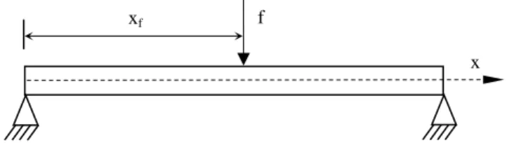
To validate the proposed formulation and its implementation, a number of numerical examples are now presented. The first and second examples demonstrate the applications of the proposed method to static analysis of simply supported beams and rectangular plates subjected to concentrated point loads. These numerical examples are presented herein to better understand the main source of er-rors in the method and to better verify the accuracy and convergence of the method. The third example is of moving load problem of beams while the last one is that of rectangular plates. Two boundary conditions, namely, fully simply supported and fully clamped end conditions are consid-ered in the third and last examples. For beams and plates with simply supported end conditions, analytical solutions can be found in the literature (Timoshenko and Woinowsky-Krieger, 1959; Fryba, 1999). Therefore, the accuracy of the proposed method can be veri ed by comparing the calculated results with those of analytical ones.
6.1 Deflection of a Simply Supported Beam Due to a Concentrated Point Load
Consider the bending problem of a simply supported beam with length L and flexural stiffness EI
Latin A m erican Journal of Solids and Structures 12 (2015) 1241-1265
Figure 2: Simply-supported beam with a concentrated point load.
The governing differential equation for the bending of the beam can be written from Eqs. (11) and (12) as
2
2 4
4 ( )
exp )
( d
) ( d
f
f
x x f
x x f x
x w
EI (30)
The procedure for discretizing Eq. (30) using the DQM is very similar to that described in Section 4. By applying the DQM to Eq. (30) we obtain
} { } ]{
[K W F (31)
where the stiffness matrix [K] is defined already in Eq. (14), and
T n x w x
w x
w( ) ( ) . . . ( )]
[ }
{W 1 2 (32)
} { }
{F f δ (33)
wherein
T f n f
f x x x x
x x
2
2 2
2 2 2
2
1 ) exp ( ) . . . exp ( )
( exp 1 } {
δ (34)
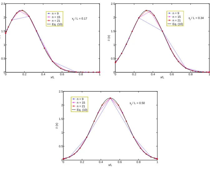
It may be seen from Eqs. (33) and (34) that the elements of the load vector{F}depend directly on the coordinates of the grid points. This implies that the coordinates of the grid points can directly affect the values of the load vector. We will show in this section that the accuracy of the solutions may also be influenced by the grid points distribution. To demonstrate this, we computed the ele-ments of the vector }{δ using Eqs. (34) and (8) for different values of xf (location of the applied load), n (number of grid points) and α (regularization parameter), and compared the results with those obtained using Eq. (10). Figures 3 and 4 illustrate the results. These results are obtained us-ing two different values of α, namely, α = 0.25 and α = 0.05.
When α = 0.25, Figure 3 compares the results of discrete model with those of the continuous
model. It can be seen that, except for n = 9, the discrete model shows a good representation to the continuous model. Note that the peak point of the discrete model with n = 9 differs slightly from that of the continuous model for xf / L = 0.17 and xf / L = 0.34. This is because the location of the applied load does not coincide with the DQM grid points in these cases.
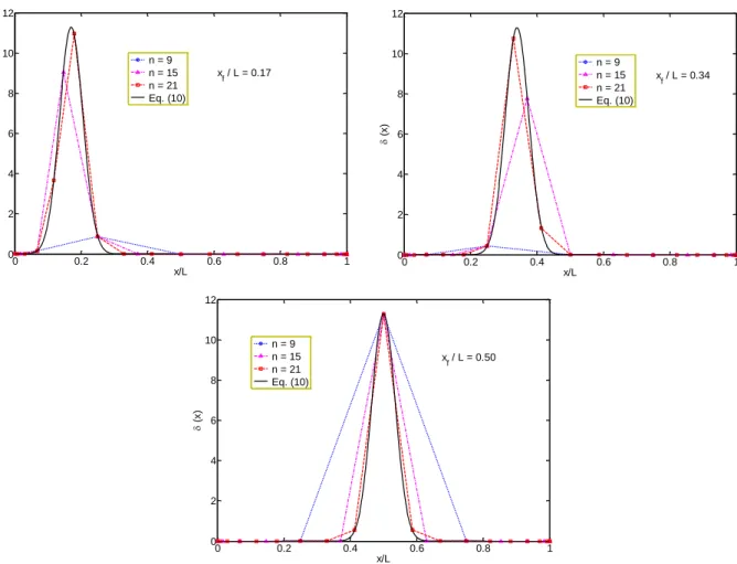
Figure 4 presents the results for α = 0.05. It can be seen from Figure 4 that when the number of
grid points is small, the discretized regularized Dirac-delta function does not provide a good
repre-x f
Latin A m erican Journal of Solids and Structures 12 (2015) 1241-1265 sentation to the original continuous function. Most importantly, the nonzero zone of the original continuous function is not accurately represented in the discretized model when the grid number is small. However, by increasing the grid number, the nonzero zone is better represented in the discre-tized model. On the other hand, by comparing the results of Figure 4 with those of Figure 3, one may conclude that as the parameter α increases, the discretized model provide better representation to the original continuous model.
Figure 3: Comparison of the discretized regularized Dirac-delta function (see Eq. (34)) with the continuous regular-ized Dirac-delta function (see Eq. (10)) for different number of grid points and locations of applied load (α = 0.25).
0 0.2 0.4 0.6 0.8 1
0 0.5 1 1.5 2 2.5
x/L
(
x
)
n = 9 n = 15 n = 21 Eq. (10)
xf / L = 0.17
0 0.2 0.4 0.6 0.8 1
0 0.5 1 1.5 2 2.5
x/L
(
x
)
n = 9 n = 15 n = 21 Eq. (10)
xf / L = 0.34
0 0.2 0.4 0.6 0.8 1
0 0.5 1 1.5 2 2.5
x/L
(
x
)
n = 9 n = 15 n = 21 Eq. (10)
Latin A m erican Journal of Solids and Structures 12 (2015) 1241-1265
0 0.2 0.4 0.6 0.8 1
0 2 4 6 8 10 12
x/L
(
x
)
n = 9 n = 15 n = 21 Eq. (10)
xf / L = 0.50
Figure 4: Comparison of the discretized regularized Dirac-delta function (see Eq. (34)) with the continuous regular-ized Dirac-delta function (see Eq. (10)) for different number of grid points and locations of applied load (α = 0.05).
As we discussed earlier in Section 3, the inappropriate choice of parameter α may be a source of error in the numerical results. This error, however, can be easily controlled by changing the value of
the regularization parameter α. On the other hand, the numerical results presented in Figures 3 and
4 show that there is another source of error (say the main source of error) which may significantly influence the accuracy of the solutions. This error is mainly due to inappropriate representation of the regularized Dirac-delta function in the discretized form.
First, from Eq. (9) we note that the error of the DQM for approximation of w(ξ) and its deriva-tives should decrease exponentially to zero due to the presence of nth factorial in the denominator. Therefore, we expect that very high accuracy to be achieved when using a significantly small num-ber of grid points. However, when the DQM is applied to the present problem, we see from Figures 3 and 4 that the regularized Dirac-delta function is not appropriately represented in the discretized model for small number of grid points and this may introduce another source of error in the numer-ical results. As it can be seen from Figures 3 and 4, this error is mainly caused by the coordinates of the grid points and is more significant for smaller values of α. A way for overcoming this difficulty is to change the coordinates of grid points such that more grid points are clustered in the nonzero
0 0.2 0.4 0.6 0.8 1
0 2 4 6 8 10 12
x/L
(
x
)
n = 9 n = 15 n = 21 Eq. (10)
xf / L = 0.17
0 0.2 0.4 0.6 0.8 1
0 2 4 6 8 10 12
x/L
(
x
)
n = 9 n = 15 n = 21 Eq. (10)
Latin A m erican Journal of Solids and Structures 12 (2015) 1241-1265
9 11 13 15 17 19 21 23 25 27 29 31
-14 -12 -10 -8 -6 -4 -2 0 2 4
Number of grid points, n
P e rc e n t e rr o r i n d im e n s io n le s s d e fl e c ti o n a t x / L = 3 /4 x
f / L = 0.15
x
f / L = 0.25
xf / L = 0.35 xf / L = 0.45
zone, for instance by stretching the grid points toward the location of the applied load. However, our numerical experiments showed that this may results in ill-conditioning of the DQM resultant matrices (to save the space, these results are not presented herein).
To demonstrate the convergence and accuracy of the proposed approach, the bending problem of a simply supported beam under a concentrated point load is solved using the proposed approach for different locations of the applied load (xf) and for two different values of the regularization
parame-ter (α). Figures 5 and 6 present the variations of the percent error in numerical solutions (defined as 100
Exact Exact
DQM w w
w ) with n for different values of xf.
The numerical results for α = 0.25 are shown in Figure 5. As it can be seen, the obtained sol u-tions converge to their final values uniformly. However, the numerical accuracy of the soluu-tions is not very satisfactory as the maximum error in the numerical results is about 17 %. This is because
the case α = 0.25 does not provide a good approximation to the original Dirac-delta function (see
Figure 1 for more details). It can also be seen from Figure 5 that, in most cases, the error in numer-ical results increases as the value of xf increases. But, the error in different points of the beam (i.e.,
x/L = 1/5, 1/2, 2/3, and 3/4) is almost the same order.
Figure 5: Convergence and accuracy of the dimensionless deflection (w/ , = fL3/EI) of a simply supported beam subjected to a concentrated point load for different locations of the applied load (α = 0.25)
9 11 13 15 17 19 21 23 25 27 29 31
-17 -16 -15 -14 -13 -12 -11 -10 -9 -8
Number of grid points, n
P e rc e n t e rr o r i n d im e n s io n le s s d e fl e c ti o n a t x / L = 1 /5 x
f / L = 0.15
x
f / L = 0.25
x
f / L = 0.35
xf / L = 0.45
9 11 13 15 17 19 21 23 25 27 29 31
-16 -14 -12 -10 -8 -6 -4 -2 0 2
Number of grid points, n
P e rc e n t e rr o r i n d im e n s io n le s s d e fl e c ti o n a t x / L = 1 /2 x
f / L = 0.15
x
f / L = 0.25
xf / L = 0.35 xf / L = 0.45
9 11 13 15 17 19 21 23 25 27 29 31
-14 -12 -10 -8 -6 -4 -2 0 2 4
Number of grid points, n
P e rc e n t e rr o r i n d im e n s io n le s s d e fl e c ti o n a t x / L = 2 /3
xf / L = 0.15 xf / L = 0.25 x
f / L = 0.35
x
Latin A m erican Journal of Solids and Structures 12 (2015) 1241-1265
9 11 13 15 17 19 21 23 25 27 29 31
-100 -50 0 50 100 150 200
Number of grid points, n
P e rc e n t e rr o r i n d im e n s io n le s s d e fl e c ti o n a t x / L = 1 /5 x
f / L = 0.15
x
f / L = 0.25
x
f / L = 0.35
xf / L = 0.45
9 11 13 15 17 19 21 23 25 27 29 31
-100 -50 0 50 100 150 200
Number of grid points, n
P e rc e n t e rr o r i n d im e n s io n le s s d e fl e c ti o n a t x / L = 1 /2 x
f / L = 0.15
xf / L = 0.25 xf / L = 0.35 x
f / L = 0.45
9 11 13 15 17 19 21 23 25 27 29 31
-100 -50 0 50 100 150 200
Number of grid points, n
P e rc e n t e rr o r i n d im e n s io n le s s d e fl e c ti o n a t x / L = 2 /3
xf / L = 0.15 xf / L = 0.25 x
f / L = 0.35
x
f / L = 0.45
9 11 13 15 17 19 21 23 25 27 29 31
-100 -50 0 50 100 150 200
Number of grid points, n
P e rc e n t e rr o r i n d im e n s io n le s s d e fl e c ti o n a t x / L = 3 /4
xf / L = 0.15 x
f / L = 0.25
x
f / L = 0.35
x
f / L = 0.45
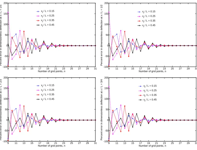
Figure 6: Convergence and accuracy of the dimensionless deflection (w/ , = fL3/EI) of a simply supported beam subjected to a concentrated point load for different locations of the applied load (α = 0.05)
Figure 6 illustrates the results for α = 0.05. It can be seen from Figure 6 that when the number of
grid points is too small, the error in quadrature solutions is very high and its behavior is oscillatory. Particularly, erroneous results are obtained when n = 9, 11, 13, and 15. As we discussed earlier, the reason for such trend of solutions is the inappropriate representation of the regularized Dirac-delta function in the discretized model for small number of grid points (see Figure 4 for details). Howev-er, the error in quadrature solutions approaches to zero rapidly by increasing the number of grid points. On the other hand, from the numerical results presented in Figure 6, one sees that the error in quadrature solutions is also influenced by the location of the applied load, as to be expected. From Figure 6, one also sees that the quadrature solutions at different points of the beam (i.e., x/L
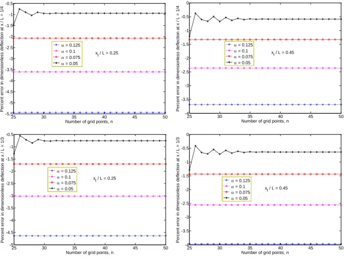
Latin A m erican Journal of Solids and Structures 12 (2015) 1241-1265 In Figure 7, the percent error in numerical results is plotted against the number of grid points
for different values of α and xf. It can be seen that the error in numerical results converges to a con-stant nonzero value by increasing the number of grid points. This nonzero concon-stant value is, in fact, the error of the regularization function (see Eq. (10)). It is clear from Figure 7 that the value of this error can be decreased significantly by decreasing the value of α.
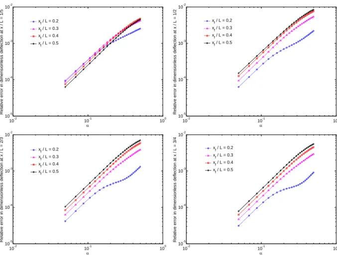
To better see the effects of regularization parameter on accuracy and convergence of solutions, the relative error in numerical results (defined aswDQM wExact ) is plotted against α in Figure 8 for different values of xf. These results are obtained using a sufficiently large number of grid points (n = 45) and are given at different points of the beam. Note that the values of α in the plot are in the range 0.05 to 0.5. As it can be seen, depending on location of the applied load, the overall order of
convergence of the method with α is in the range 1 to 2. This implies that the employed regularized
Dirac-delta function is at most second-order accurate. On the other hand, the results of Figure 8 show that the order of convergence of the method (with respect to α) depends on the location of the applied load, and increases as xf → 0.5.
Figure 7: Convergence and accuracy of the dimensionless deflection (w/ , = fL3/EI) of a simply supported beam subjected to a concentrated point load for different values of α.
25 30 35 40 45 50
-5.5 -5 -4.5 -4 -3.5 -3 -2.5 -2 -1.5 -1 -0.5
Number of grid points, n
P e rc e n t e rr o r i n d im e n s io n le s s d e fl e c ti o n a t x / L = 1 /4
= 0.125 = 0.1 = 0.075 = 0.05
xf / L = 0.25
25 30 35 40 45 50
-4 -3.5 -3 -2.5 -2 -1.5 -1 -0.5 0
Number of grid points, n
P e rc e n t e rr o r i n d im e n s io n le s s d e fl e c ti o n a t x / L = 1 /4
= 0.125 = 0.1 = 0.075 = 0.05
x
f / L = 0.45
25 30 35 40 45 50
-5 -4.5 -4 -3.5 -3 -2.5 -2 -1.5 -1 -0.5
Number of grid points, n
P e rc e n t e rr o r i n d im e n s io n le s s d e fl e c ti o n a t x / L = 1 /3
= 0.125 = 0.1 = 0.075 = 0.05
x
f / L = 0.25
25 30 35 40 45 50
-4 -3.5 -3 -2.5 -2 -1.5 -1 -0.5 0
Number of grid points, n
P e rc e n t e rr o r i n d im e n s io n le s s d e fl e c ti o n a t x / L = 1 /3
= 0.125 = 0.1 = 0.075 = 0.05
Latin A m erican Journal of Solids and Structures 12 (2015) 1241-1265
Figure 8: Variations of relative error in numerical results with α for different locations of the applied load (n = 45)
6.2 Deflection of a Simply Supported Rectangular Plate Due to a Concentrated Point Load
Consider the bending problem of a simply supported rectangular plate with length a, width b, thickness h, and bending stiffness D subjected to a concentrated transverse load f acting at a point (x, y) = (xf, yf). The governing differential equation for the bending of the plate can be written from Eqs. (18) and (19) as
2 2 2 2 2 4 4 2 2 4 4
4 ( )
exp ) ( exp 2
f f
y y x x f y w y x w x w D (35)
The procedure for discretizing Eq. (35) using the DQM is very similar to that described in Section 5 and is not repeated here again.
Our numerical results for the present problem showed that the error in numerical results may have similar trend as that shown in Figures 5 and 6 for the beam problem. Most importantly, the
convergence problem of the method for the case of small values of α and n has been found to be
more critical than that of the beam problem due to the existence of the double Dirac-delta function in the governing differential equation of the plate. This can be clearly observed from the numerical
10-2 10-1 100
10-5 10-4 10-3 10-2 Rel a ti v e e rr o r i n d im e n s io n le s s d e fl e c ti o n a t x / L = 1 /5 x
f / L = 0.2
x
f / L = 0.3
xf / L = 0.4 xf / L = 0.5
10-2 10-1 100
10-5 10-4 10-3 10-2 Rel a ti v e e rr o r i n d im e n s io n le s s d e fl e c ti o n a t x / L = 1 /2 x
f / L = 0.2
xf / L = 0.3 x
f / L = 0.4
x
f / L = 0.5
10-2 10-1 100
10-5 10-4 10-3 10-2 Rel a ti v e e rr o r i n d im e n s io n le s s d e fl e c ti o n a t x / L = 2 /3
xf / L = 0.2 xf / L = 0.3 x
f / L = 0.4
x
f / L = 0.5
10-2 10-1 100
10-5 10-4 10-3 10-2 Rel a ti v e e rr o r i n d im e n s io n le s s d e fl e c ti o n a t x / L = 3 /4
xf / L = 0.2 x
f / L = 0.3
x
f / L = 0.4
x
Latin A m erican Journal of Solids and Structures 12 (2015) 1241-1265
15 20 25 30 35
-50 0 50 100
Number of grid points, n = m
Pe rce n t e rro r in d ime n si o n le ss d e fl e ct io n a t (x / a , y / b ) = (1 /4 , 1 /3 )
= 0.125
= 0.1
= 0.075
= 0.05
(xf / a, yf / b) = (0.25, 0.5)
15 20 25 30 35
-18 -16 -14 -12 -10 -8 -6 -4 -2 0 2
Number of grid points, n = m
Pe rce n t e rro r in d ime n si o n le ss d e fl e ct io n a t (x / a , y / b ) = (1 /4 , 1 /3 )
= 0.125
= 0.1
= 0.075
= 0.05
(xf / a, yf / b) = (0.45, 0.5)
10-2 10-1 100
10-5 10-4 10-3 10-2 R e la ti ve e rro r in d ime n si o n le ss d e fl e ct io n a t (x / a , y / b ) = (1 /3 , 1 /3 )
(xf / a, yf / b) = (0.2, 0.5) (xf / a, yf / b) = (0.3, 0.5)
(xf / a, yf / b) = (0.4, 0.5)
(xf / a, yf / b) = (0.5, 0.5)
10-2 10-1 100
10-5 10-4 10-3 10-2 R e la ti ve e rro r in d ime n si o n le ss d e fl e ct io n a t (x / a , y / b ) = (3 /4 , 3 /4 )
(xf / a, yf / b) = (0.2, 0.5)
(xf / a, yf / b) = (0.3, 0.5) (xf / a, yf / b) = (0.4, 0.5) (xf / a, yf / b) = (0.5, 0.5)
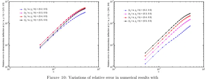
results presented in Figure 9.The effects of regularization parameter value on accuracy and conver-gence of the solutions are studied in Figure 10. Again, one sees that the regularization function (10) is at most second-order accurate.
Figure 9: Convergence and accuracy of the dimensionless deflection (w/ , = fa2/D) of a simply supported square plate subjected to a concentrated point load for different values of α.
Figure 10: Variations of relative error in numerical results with respect to α for different locations of the applied load (n = m = 45)
6.3 Vibration of a Beam Due to a Moving Point Load
Consider a simply supported beam with a span L of 10.16 cm, width b = 0.635 cm, thickness h = 0.635 cm, modulus of elasticity E = 2.068 × 10¹¹ Pa, mass density ρ = 10686.9 kg/m3, subjected to a f = 4.45 N moving force (Rieker et al., 1996). The dynamic responses at the beam center, wcd, are evaluated for different values of v (velocity of moving load) and normalized by the static deflection
Latin A m erican Journal of Solids and Structures 12 (2015) 1241-1265
Our numerical experiments for the present problem showed that the value of α at which the
convergence is attained depends considerably on the value of the beam length. Particularly, for very short beams, the numerical convergence has been achieved using only too small values of α. This phenomenon can be easily justified from the results presented in Figure 1, wherein the variations of the regularized Dirac-delta function versus x are shown. From Figure 1, we see that the regularized Dirac-delta function has nonzero values at x < 0.2 for every value of α 0.0625. This implies that for the case of beams with L < 0.2, one should use very small values of α in the method to insure
the convergence and accuracy of the solutions (α << 0.0625).
A way for overcoming the above-mentioned drawback is to express the governing differential equation of the beam in dimensionless form such that the domain of the problem is changed from 0
x L to 0 X 1. Then a similar procedure as that explained in Section 4 can be applied to discretize the resulting non-dimensional differential equation. By doing so, larger values of α can be used in the method, as we will show in the following (This can also be seen from the numerical re-sults of the static analysis (see Figures 5-8)). By introducing the dimensionless variable X = x/L, the governing differential equation of motion of the beam can be written from Eq. (11) as
)), ( (
) , ( ) ,
( 3
4 4 2
2 4
t X X EI fL X
t X w t
t X w EI AL
f
L
v t L
t x t
X f
f ) ( )
( (36)
Now, introducing the regularized Dirac-delta function (10) to Eq. (36) gives
2 2 2
4 4 2
2 1
)) ( (
exp )
, ( ) , (
X X t
X t X w t
t X
w f
(37)
where
,
4 1
EI AL
EI
fL3 2
(38)
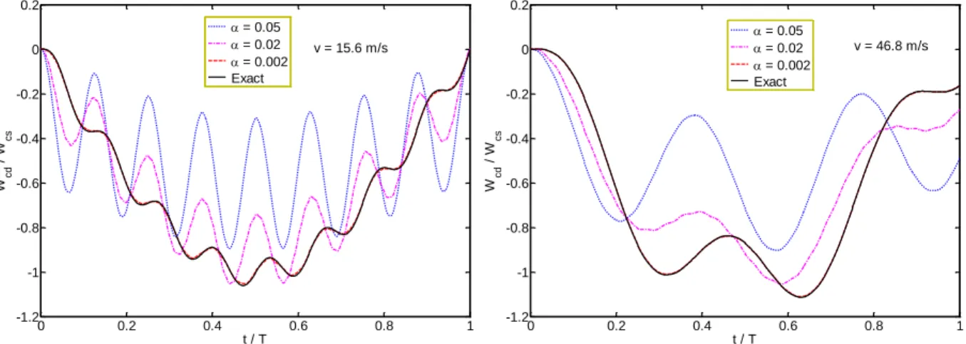
Figures 11 and 12 show the effect of regularization parameter, α, on accuracy and convergence of
the results for two different values of moving speed. The analytical solution values are also shown for comparison. Note that the numerical results are shown for two different cases: (i) the case where
the dimensional differential equation of the beam is considered (see Eq. (12)); and (ii) the case
where the dimensionless differential equation of the beam is considered (see Eq. (37)). As it can be seen from Figures 11 and 12, the results of case (i) are not very satisfactory in terms of both accu-racy and convergence. The results of case (ii) are found to be more superior to those of case (i), particularly in terms of numerical convergence. Note that when case (ii) is considered, better
Latin A m erican Journal of Solids and Structures 12 (2015) 1241-1265
0 0.2 0.4 0.6 0.8 1
-1.2 -1 -0.8 -0.6 -0.4 -0.2 0 0.2
t / T
W
c
d
/ W
c
s
= 0.05
= 0.02
= 0.002 Exact
v = 15.6 m/s
0 0.2 0.4 0.6 0.8 1
-1.2 -1 -0.8 -0.6 -0.4 -0.2 0 0.2
t / T
W
c
d
/ W
c
s
= 0.05
= 0.02
= 0.002 Exact
v = 46.8 m/s
Figure 11: Convergence and accuracy of the numerical results with decreasing α-value for the case where the di-mensional differential equation of motion of the beam is discretized using the DQM (n = 51).
Figure 12: Convergence and accuracy of the numerical results with decreasing α-value for the case where the dimensionless differential equation of motion of the beam is discretized using the DQM (n = 51).
On the other hand, from numerical results presented in Figure 12, one sees the rate of convergence
of the method with α increases as the load speed increases. Therefore, larger values of α can be used in the method for the case of high speed of travelling load. Figure 13 shows the convergence of solu-tions with respect to the number of grid points (n). It can be seen from Figure 13 that the results of proposed method converge uniformly and agree well with the analytical solutions. It can also be clearly seen from this figure that the rate of convergence of the method with n increases as the load speed increases. This implies that smaller number of grid points can be used in the method for the case of high speed of travelling load.
0 0.2 0.4 0.6 0.8 1
-1.2 -1 -0.8 -0.6 -0.4 -0.2 0 0.2
t / T
W
c
d
/ W
c
s
= 0.075
= 0.05
= 0.025 Exact
v = 15.6 m/s
0 0.2 0.4 0.6 0.8 1
-1.2 -1 -0.8 -0.6 -0.4 -0.2 0 0.2
t / T
W
c
d
/ W
c
s
= 0.075
= 0.05
= 0.025 Exact
Latin A m erican Journal of Solids and Structures 12 (2015) 1241-1265
Figure 13: Convergence and accuracy of numerical results for normalized central deflection of a simply supported beam subjected to a moving load for different load speeds.
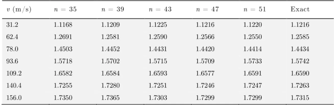
The numerical experiments are also carried out to obtain the dynamic magni cation factors (DMFs) (maximum value of normalized deflection at the beam center) for various values of moving speed. The numerical results are given in Table 1. These results are obtained using α = 0.018 and different values of n (number of grid points). The analytical solution values are also tabulated in this table for comparison purposes. It can be seen from Table 1 that the results generated by the proposed method converge rapidly and agree very closely with the analytical solutions.
v (m/s) n = 35 n = 39 n = 43 n = 47 n = 51 Exact
31.2 1.1168 1.1209 1.1225 1.1216 1.1220 1.1216
62.4 1.2691 1.2581 1.2590 1.2566 1.2550 1.2585
78.0 1.4503 1.4452 1.4431 1.4420 1.4414 1.4434
93.6 1.5718 1.5702 1.5715 1.5709 1.5733 1.5742
109.2 1.6582 1.6584 1.6593 1.6577 1.6591 1.6590
140.4 1.7255 1.7280 1.7251 1.7246 1.7247 1.7263
156.0 1.7350 1.7365 1.7303 1.7299 1.7299 1.7315
Table 1: Convergence and accuracy of DMFs of a simply supported beam subjected to a moving concentrated load for different load speeds (α = 0.018).
Now, consider a moving point load on a beam with clamped-clamped boundary conditions. Alt-hough analytical solutions do not exist for this condition, accurate numerical solutions are available in the literature (Rieker et al., 1996). Therefore, the accuracy of the method can also be checked for this case. The dynamic responses at the beam center are evaluated for different travel speeds (v)
and normalized by the static de ection wcs = fL3/(192EI) of a fully clamped beam under a point
load f at mid-span. The numerical results are tabulated in Tables 2 and 3 together with the finite
0 0.2 0.4 0.6 0.8 1
-1.2 -1 -0.8 -0.6 -0.4 -0.2 0 0.2
t / T
W
c
d
/ W
c
s
n = 35 n = 39 n = 43 Exact
v = 15.6 m/s, = 0.025
0 0.2 0.4 0.6 0.8 1
-1.2 -1 -0.8 -0.6 -0.4 -0.2 0 0.2
t / T
W
c
d
/ W
c
s
n = 29 n = 33 n = 37 Exact
Latin A m erican Journal of Solids and Structures 12 (2015) 1241-1265 element solutions obtained by Rieker et al. (1996). Note that these results are obtained using two
different values of α. Excellent agreements are observed between the results of present analysis and
those of Rieker et al. (1996). Besides, the convergence behavior of solutions is more uniform in the
case α = 0.025 as compared with the case α = 0.02. However, the accuracy of the solutions in the
case α = 0.02 is better than that in the case α = 0.025. From the numerical results presented in this
section, it can be concluded that the proposed approach is very well suitable for handling the mov-ing load problem on beam-like structures.
v (m/s) n = 31 n = 33 n = 35 n = 37 n = 39 R ieker et al. (1996)
141.3070 1.303 1.304 1.302 1.301 1.301 1.311 282.6140 1.629 1.633 1.632 1.632 1.633 1.637 423.9210 1.546 1.553 1.551 1.548 1.547 1.552
Table 2: Convergence and accuracy of DMFs of a clamped beam subjected
to a moving concentrated load for different load speeds (α = 0.025).
v (m/s) n = 31 n = 33 n = 35 n = 37 n = 39 R ieker et al. (1996)
141.3070 1.308 1.313 1.307 1.303 1.303 1.311 282.6140 1.630 1.636 1.636 1.634 1.636 1.637 423.9210 1.548 1.559 1.556 1.551 1.549 1.552
Table 3: Convergence and accuracy of DMFs of a clamped beam subjected
to a moving concentrated load for different load speeds (α = 0.02).
6.4 Vibration of a Rectangular Plate Due to a Moving Point Load
To demonstrate the applicability of the proposed method for the forced vibration analysis of rectan-gular plates carrying moving dynamic loads, application is made to a numerical example given by Eftekhari and Jafari (2012d). The parameters used in this numerical example are as follows:
ρh/D = 1, f/D = 1, a = b = 1, xf(t) = vt, yf(t) = constant = ½
where v is the velocity of the moving load in the x-direction and t is the time. Other parameters are defined already in Section 5. As pointed out earlier, an analytical solution for the present problem is given in Fryba (1999) for plates with simply supported end conditions which will be used here to validate the proposed method. Figure 14 demonstrates the influence of the regularization parameter,
α, on the accuracy of solutions and Figure 15 shows the convergence behavior of solutions with
Latin A m erican Journal of Solids and Structures 12 (2015) 1241-1265
0 0.2 0.4 0.6 0.8 1 1.2 1.4
-14 -12 -10 -8 -6 -4 -2 0 2x 10
-3
t: sec
C
e
n
tr
a
l
d
e
fl
e
c
ti
o
n
:
m
= 0.3
= 0.075
= 0.03 Exact
v = 0.75 m/s
0 0.1 0.2 0.3 0.4 0.5
-18 -16 -14 -12 -10 -8 -6 -4 -2 0 2x 10
-3
t: sec
C
e
n
tr
a
l
d
e
fl
e
c
ti
o
n
:
m
n = m = 35 n = m = 39 n = m = 43 Exact
v = 2 m/s Figure 14: Effect of α-value on the accuracy of numerical results for central deflection of a simply
supported square plate subjected to a moving load for different load speeds (n = m = 45).
Figure 15: Convergence and accuracy of numerical results for central deflection of a simply supported square plate subjected to a moving load for different load speeds (α = 0.03).
It can be seen from Figure 14 that the accuracy of solutions is improved significantly by decreasing
the magnitude of α. On the other hand, by comparing these results with those of static analysis (see
Figures 9 and 10), one sees that a smaller value of α should be used in the dynamic analysis of plates. For instance, as it can be seen from Figure 9, an acceptable accurate solutions for the static analysis of plates are achieved using α = 0.05. This value for the dynamic analysis of plates is α = 0.03 which is slightly smaller than that of the static analysis. The reason for this may be due to accumulation of the error in the time integration scheme, noting that the location of the applied load may affect the error of numerical results at each time step (see Figures 9 and 10 for more de-tails).
Now, consider a moving point load on a plate with fully clamped boundary conditions. The nu-merical results for this case are presented in Figure 16. The Ritz-DQM solutions of Eftekhari and
0 0.1 0.2 0.3 0.4 0.5 0.6 0.7
-14 -12 -10 -8 -6 -4 -2 0 2x 10
-3
t: sec
C
e
n
tr
a
l
d
e
fl
e
c
ti
o
n
:
m
= 0.3
= 0.075
= 0.03 Exact
v = 1.5 m/s
0 0.2 0.4 0.6 0.8 1
-14 -12 -10 -8 -6 -4 -2 0 2x 10
-3
t: sec
C
e
n
tr
a
l
d
e
fl
e
c
ti
o
n
:
m
n = m = 35 n = m = 39 n = m = 43 Exact
Latin A m erican Journal of Solids and Structures 12 (2015) 1241-1265
0 0.2 0.4 0.6 0.8 1
-6 -5 -4 -3 -2 -1 0 1x 10
-3
t: sec
C
e
n
tr
a
l
d
e
fl
e
c
ti
o
n
:
m
n = m = 41 n = m = 43 n = m = 45 Ritz-DQM
v = 1 m/s
0 0.02 0.04 0.06 0.08 0.1 0.12 0.14 0.16 0.18
-9 -8 -7 -6 -5 -4 -3 -2 -1 0 1x 10
-3
t: sec
C
e
n
tr
a
l
d
e
fl
e
c
ti
o
n
:
m
n = m = 33 n = m = 37 n = m = 41 Ritz-DQM
v = 6 m/s
Jafari (2012d) are also shown for comparison. It can be seen that the results of proposed method converge smoothly and agree well with those of the Ritz-DQM.
Figure 16: Convergence and accuracy of numerical results for central deflection of a clamped square plate subjected to a moving load for different load speeds (α = 0.03).
7 CONCLUSIONS
There are many problems in applied mechanics whose governing partial differential equations in-volve the Dirac-delta function. For instance, the behavior of structures under impulsive loading, the static and dynamic behavior of structures under impact loading, the thermoelastic dynamic behav-ior of structures under heat or pressure point sources can be mathematically described by means of the Dirac-delta function. In each of these problems, the accurate prediction of the structure re-sponse is very important and is a key factor in the design and analysis of such structures. In gen-eral, such type of problems can be solved by the help of analytical and/or numerical methods. Among the numerical methods, the point discretization techniques such as the collocation, finite difference, discrete singular convolution, and the differential quadrature methods have been success-fully applied by many researchers to various problems encountered in applied mechanics.
Latin A m erican Journal of Solids and Structures 12 (2015) 1241-1265
The main advantage of the proposed method is its simplicity. Most importantly, the proposed method can be used as an efficient tool for the dynamic analysis of plates under loads moving along an arbitrary trajectory on the plate surface.
References
Bathe, K.J., Wilson, E.L. (1976). Numerical Methods in Finite Element Analysis. Prentice-Hall, Englewood Cliffs (New Jersey).
Bellman, R.E., Casti, J. (1971). Differential quadrature and long term integration. J Math Anal Appl 34: 235–238. Bellman, R.E., Kashef, B.G., Casti, J. (1972). Differential quadrature: A technique for the rapid solution of nonlinear partial differential equations. J Comput Phys 10: 40–52.
Bert, C.W., Malik, M. (1996a). Differential quadrature method in computational mechanics: A review. ASME Appl Mech Rev 49: 1–28.
Bert, C.W., Malik, M. (1996b). The differential quadrature method for irregular domains and application to plate vibration. Int J Mech Sci 38(6): 589-606.
Burko, L.M., Khanna, G. (2007). Accurate time–domain gravitational waveforms for extreme-mass-ratio binaries. Europhys Lett 78: 60005.
Civalek, Ö. (2004). Application of differential quadrature (DQ) and harmonic differential quadrature (HDQ) for buckling analysis of thin isotropic plates and elastic columns. Eng Struct 26(2):171-186.
Eftekhari, S.A., Jafari, A.A. (2012a). Numerical simulation of chaotic dynamical systems by the method of differen-tial quadrature. Sci Iran B 19(5): 1299–1315.
Eftekhari, S.A., Jafari, A.A. (2012b) Vibration of an initially stressed rectangular plate due to an accelerated travel-ing mass. Sci Iran A 19(5):1195–1213.
Eftekhari, S.A., Jafari, A.A. (2012c) Mixed nite element and di erential quadrature method for free and forced
vibration and buckling analysis of rectangular plates. Appl Math Mech 33(1):81–98.
Eftekhari, S.A., Jafari, A.A. (2012d) A mixed method for free and forced vibration of rectangular plates. Appl Math Model 36: 2814–2831.
Eftekhari, S.A., Jafari, A.A. (2014). A mixed modal-differential quadrature method for free and forced vibration of
beams in contact with uid. Meccanica 49:535–564.
Engquist, B., Tornberg, A-K., Tsai, R. (2005). Discretization of Dirac delta functions in level set methods. J Comput Phys 207: 28–51.
Fryba, L. (1999). Vibration of Solids and Structures under Moving Loads. Thomas Telford (London).
Gheorghiu, C.I. (2007). Spectral Methods for Differential Problems. Casa Cartii de Stiinta Publishing House, Cluj-Napoca.
Jung, J-H. (2009). A Note on the spectral collocation approximation of some differential equations with singular source terms. J Sci Comput 39: 1573–7691.
Jung, J-H., Don, W.S. (2009). Collocation methods for hyperbolic partial differential equations with singular sources. Adv Appl Math Mech 1(6):769-780.
Jung, J-H., Khanna, G. Nagle, I. (2009). A spectral collocation approximation for the radial-infall of a compact ob-ject into a Schwarzschild black hole. Int J Mod Phys C 20:1–22.
Kananipour, H., Ahmadi, M., Chavoshi, H. (2014). Application of nonlocal elasticity and DQM to dynamic analysis of curved nanobeams. Latin American J Solids Struct 11: 848-853.
Latin A m erican Journal of Solids and Structures 12 (2015) 1241-1265 Malik, M., Bert, C.W. (1996). Implementing multiple boundary conditions in the DQ solution of higher-order PDE’s:
application to free vibration of plates. Int J Numer Meth Eng 39:1237-1258.
Nikkhoo, A., Kananipour, H., Chavoshi, H., Zarfam, R. (2012). Application of differential quadrature method to investigate dynamics of a curved beam structure acted upon by a moving concentrated load. Indian J Sci Technol 5: 3085–3089.
Nikkhoo, A., Kananipour, H. (2014). Numerical solution for dynamic analysis of semicircular curved beams acted upon by moving loads. Proc IMechE Part C: J Mech Eng Sci doi: 10.1177/0954406213518908.
Quan, J.R., Chang, C.T. (1989). New insights in solving distributed system equations by the quadrature methods, Part I: analysis. Comput Chem Eng 13:779–788.
Rao, S.S. (2007). Vibration of Continuous Systems. John Wiley & Sons, Inc. (New Jersey).
Rieker, J. R., Lin, Y.-H., Trethewey, M. W. (1996). Discretization considerations in moving load finite element beam models. Finite Elem Anal Design 21: 129–144.
Rivera, M.J., Trujillo, M., Romero-García, V., López Molina, J.A., Berjano, E. (2013). Numerical resolution of the hyperbolic heat equation using smoothed mathematical functions instead of Heaviside and Dirac delta distributions. Int Commun Heat Mass Trans 46: 7 –12.
Shu, C. (1996) Free vibration analysis of composite laminated conical shells by generalized differential quadrature. J Sound Vib 194(4): 587–604.
Shu, C., Du, H. (1997a). Implementation of clamped and simply supported boundary conditions in the GDQ free vibration analysis of beams and plates. Int J Solids Struct 34(7):819-835.
Shu, C., Du, H. (1997b). A generalized approach for implementing general boundary conditions in the GDQ free vibration analyses of plates. Int J Solids Struct 34(7): 837–846.
Shu, C. (2000). Differential Quadrature and Its Application in Engineering. Springer (New York).
Sundararajan, P.A., Khanna, G., Hughes, S.A. (2007).Towards adiabatic waveforms for inspiral into Kerr black holes: I. A new model of the source for the time domain perturbation equation. Phys Rev D 76: 104005.
Timoshenko, S.P., Woinowsky-Krieger, S. (1959). Theory of Plates and Shells. McGraw-Hill (New York).
Towers, D. (2007). Two methods for discretizing a delta function supported on a level set. J Comput Phys 220: 915–
931.
Waldén, J. (1999). On the approximation of singular source terms in differential equations. Numer Methods Partial Diff Eqs 15: 503–520.
Wang, X., Bert, C.W., Striz, A.G. (1993). Di erential quadrature analysis of de ection, buckling, and free vibration
of beams and rectangular plates. Comput Struct 48(3): 473–479.
Wang, D., Jung, J-H., Biondini, G. (2014). Detailed comparison of numerical methods for the perturbed sine-Gordon equation with impulsive forcing. J Eng Math doi: 10.1007/s10665-013-9678-x.
Wei, G.W., Zhao, Y.B., Xiang, Y. (2002). Discrete singular convolution and its application to the analysis of plates with internal supports, Part 1: Theory and algorithm. Int J Numer Meth Eng 55 :913–946.