Abstract
In this paper, forming limit diagrams (FLDs) for an aluminum alloy are predicted through numerical simulations using various localized necking criteria. A comparative study is conducted for the FLDs determined by using the Lemaitre damage approach and those obtained with the modified Gurson–Tvergaard–Needleman (GTN) damage model. To this end, both damage models coupled with elasto-plasticity and accounting for plastic anisotropy have been implemented into the ABAQUS/Explicit software, through the user-defined subroutine VUMAT, within the framework of large plastic strains and a fully three-dimensional formulation. The re-sulting constitutive frameworks are then combined with four local-ized necking criteria to predict the limit strains for an AA6016-T4 aluminum alloy. Three of these necking criteria are based on finite element (FE) simulations of the Nakazima deep drawing test with various specimen geometries, while the fourth criterion is based on bifurcation theory. The simulation results reveal that the limit strains predicted by local criteria, which are based on FE simula-tions of the Nakazima test, are in good agreement with the experi-ments for a number of strain paths, while those obtained with the bifurcation analysis provide an upper bound to the experimental FLD.
Keywords
GTN model, Lemaitre damage approach, plastic anisotropy, form-ing limit diagram, localized neckform-ing criteria, bifurcation theory, Nakazima deep drawing test.
Determination of Forming Limit Diagrams Based
on Ductile Damage Models and Necking Criteria
1 INTRODUCTION
The good knowledge of the formability of metallic materials is very important for the successful forming of sheet metals. The concept of forming limit diagram (FLD), which was originally
intro-Hocine Chalal a, b, * Farid Abed-Meraim a, b
a LEM3, UMR CNRS 7239 – Arts et
Métiers ParisTech, 4 rue Augustin Fresnel, 57078 Metz Cedex 3, France.
b DAMAS, Laboratory of Excellence on
Design of Alloy Metals for low-mAss Structures, Université de Lorraine, France.
Email: [email protected] Email: [email protected]
* Corresponding auhor
http://dx.doi.org/10.1590/1679-78253481
duced by Keeler and Backofen (1963), and later by Goodwin (1968), has been the most widely used tool for the characterization of the formability of sheet metals. This strategy allows delimiting the limit strains for stretched sheet metals that should not be exceeded in order to ensure a good quali-ty of the final product. The FLDs are determined using necking or fracture criteria, which may be based on sound theoretical developments (see, e.g., Hill, 1952; Stören and Rice, 1975; Yamamoto, 1978; Abed-Meraim et al., 2014) or on finite element (FE) simulations (see, e.g., Zhang et al., 2011; Lumelskyy et al., 2012, Martínez-Donaire et al., 2014; Kami et al., 2015). These criteria are general-ly combined with constitutive models for the prediction of limit strains in sheet metal forming. In order to describe the behavior of sheet metals in a realistic way, advanced elastic–plastic models coupled with damage have been developed in the literature, which can be classified into two main approaches, namely the micromechanics damage modeling (MDM) and the continuum damage me-chanics (CDM). The MDM approach has been first developed by Gurson (1977), who considered the initiation of damage as the growth of micro-voids in porous materials surrounded by a rigid– plastic matrix. This preliminary modeling approach has subsequently received a number of exten-sions to obtain the so-called Gurson–Tvergaard–Needleman (GTN) damage model (see, e.g., Tvergaard, 1982a,1982b; Tvergaard and Needleman, 1984) in order to account for all damage mechanisms (i.e., nucleation, growth and coalescence of voids) as well as the hardening of the dense matrix. Concurrently, the CDM approach has been introduced by the works of Kachanov (1958), and extended later in the framework of irreversible thermodynamics (see, e.g., Lemaitre, 1992; Chaboche, 1999). In the CDM approach, the damage variable represents the surface density of mi-crocracks across a given plane, and may be modeled as an isotropic scalar variable (see, e.g., Le-maitre, 1985, 1992), or a tensor variable for anisotropic damage (see, e.g., Lemaitre et al., 2000; Brünig, 2003).
In this work, both the MDM and the CDM approaches are adopted for the modeling of ductile damage in sheet metals. More specifically, a classical elastic–plastic model with anisotropic plastici-ty is coupled with the Lemaitre damage theory, while the GTN model is combined with the Hill (1948) anisotropic yield surface to account for plastic anisotropy. The resulting models are imple-mented into the finite element code ABAQUS/Explicit, through the user-defined subroutine VUMAT, within the framework of large plastic strains and a fully three-dimensional formulation. Each of these models is then used for the FE simulations of the Nakazima deep drawing test with different specimen geometries in order to predict FLDs. The latter are determined using four differ-ent criteria for the onset of localized necking. Three of these criteria are based on the FE simula-tions of the Nakazima deep drawing test, while the fourth one is based on bifurcation theory (see, e.g., Rudnicki and Rice, 1975; Stören and Rice, 1975; Rice, 1976). The numerical FLDs obtained with the current approach are compared with the experimental results taken from Kami et al. (2015).
2 MODELING OF DUCTILE DAMAGE
2.1 GTN Damage Model
Gurson (1977) proposed a yield condition depending on the void volume fraction, which represents the density of micro-defects within the material. Subsequently, this model has been improved by Tvergaard (1981) and Tvergaard and Needleman (1984) in order to take into account the interac-tion between voids. The resulting modificainterac-tions led to the definiinterac-tion of the following plastic yield surface:
2
* *2
GTN eq
2
1cosh
3
2
2 m1
30
Y Y
σ
q f
q
σ
q f
, (1)where σeq( )σ 3 : 2σ σ is the macroscopic von Mises equivalent stress, σm 1 :3σ 1 is the
hydro-static stress, σ σ σm1 is the deviatoric part of the Cauchy stress σ, with 1 being the
second-order identity tensor. The isotropic hardening of the fully dense matrix is described by the variable
plY , function of the equivalent plastic strain pl. The parameters q1, q2 and q3, introduced by Tvergaard (1981, 1982a), account for void interaction effects. The void coalescence mechanism is considered through the introduction of an effective void volume fraction f*
f (see, e.g., Tvergaard, 1982b; Tvergaard and Needleman, 1984). This function is defined as
* *
for , ( )
for , cr
u cr
cr cr cr R
R cr
f f f
f f f f
f f f f f f
f f
(2)where f represents the actual void volume fraction, fu* is the ultimate value of f*, while fR is the void volume fraction at fracture. The void coalescence phenomenon occurs when the void vol-ume fraction reaches the critical value fcr.
In order to account for the plastic anisotropy of the material, the GTN plastic yield surface (see Eq. (1)) is modified by introducing the Hill (1948) equivalent stress instead of the von Mises one (see, e.g., Chen and Butcher, 2013; Kami et al., 2015; Li et al., 2015). The corresponding expression of equivalent stress is given by
( ) : :
eq
σ σ σ M σ , (3)
where the fourth-order tensor M contains the six anisotropy coefficients of the Hill (1948) quadrat-ic yield criterion. It is worth noting that the original isotropquadrat-ic GTN model is recovered from the anisotropic one when the Lankford coefficients r0, r45 and r90 are set to 1.
Based on the principle of equivalence in plastic work rate (Gurson, 1977), the equivalent plastic strain rate pl of the fully dense matrix material is obtained as follows:
p
pl :
1 f Y
σ D
where Dp is the macroscopic plastic strain rate tensor. The latter is defined using the classical normality rule with respect to the yield function, and is expressed as
p
GTN
λ
D V , (5)
where λ is the plastic multiplier, and VGTN ΦGTN σ is the direction of the plastic flow. Iso-tropic hardening for the dense matrix is assumed in this work, which is defined by the following expression:
pl
Yh , (6)
where h
pl is the plastic hardening modulus of the fully dense matrix material.The evolution of the void volume fraction is based on both nucleation of new voids and growth of existing voids (see, e.g., Chu and Needleman, 1980). The associated evolution equation is given by
growth nucleation
f f f , (7)
where
pgrowth 1 :
f f D 1. (8)
For the void nucleation, the latter is assumed to be strain controlled in this work. The expres-sion of the nucleation rate is given by
pl nucleation N
f A , (9)
where AN has been defined in Chu and Needleman (1980) by the following normal distribution law:
2 pl 1 exp
2 2
N N
N
N N
f A
s
s π
, (10)
where fN is the volume fraction of the inclusions that are likely to nucleate, N is the mean
equivalent plastic strain of nucleation, and sN is the corresponding standard deviation.
The consistency condition for the GTN model, which ensures plastic loading, may be written in the following form:
*
GTN GTN GTN
Φ V :σV Y +Y Vf f = 0, (11)
*
* GTN
GTN 2 1 2 2
2
* GTN
1 2 2
3 2
* GTN
1 2 3
*
Φ 2 : sinh 3
2
Φ 2 3 sinh 3
2
Φ 2 cosh 3 2
2
m
eq m m
Y
m f
σ
f
q q q
Y Y
Y
σ σ σ
V q q f q
Y Y Y Y
σ
V q q q f
Y f M σ
V = 1
σ
=
=
, (12)
and * GTN 1 for for cr u cr cr R R cr f f f f
f f f
f f
. (13)
In the co-rotational frame, which is associated with the Jaumann objective derivative, the Cau-chy stress–strain relationship is obtained using the classical hypoelastic law defined by
p
GTN = e: ep :
σ C D D C D, (14)
where Ce is the fourth-order elasticity tensor, GTN ep
C is the elastic–plastic tangent modulus for the GTN model, and D is the strain rate tensor.
By substituting Eqs. (4)–(9) into the consistency condition (11), the expression of the plastic multiplier λ is obtained as follows:
GTN GTN : : = e λ H
V C D
, (15)
where
GTN *
*GTN GTN: e: GTN 11 : Y N f GTN 1 GTN f GTN:
H hV A V f V
f Y
σ V
= V C V V 1. (16)
The analytical expression of the elastic–plastic tangent modulus for the GTN model is obtained by substituting the expression of the plastic multiplier (Eq. (15)) into the hypoelastic relationship (14)
GTN
GTN
GTN
GTN
: :
=
e e
ep e α
H
C V V C
C C , (17)
where α=0 for elastic loading/unloading, and α=1 for strict plastic loading.
2.2 Lemaitre Damage Model
is referred to as Continuum Damage Mechanics (CDM) theory, which provides a phenomenological description for ductile damage, in contrast to the micromechanics-based Gurson damage model. In the CDM theory, the damage variable, which may be scalar isotropic or tensor-valued anisotropic, represents the surface density of microdefects. In the current work, the adopted elasto-plastic model coupled with ductile damage takes into account the initial anisotropy of the material, using the Hill’48 quadratic yield function, while hardening is taken to be isotropic.
Based on the strain equivalence principle (Lemaitre and Chaboche, 1978), the material behavior is affected by continuum damage through the introduction of an effective stress tensor σ given by
= 1d
σ
σ , (18)
where the scalar damage variable d varies between 0 to 1, with d =0 for an undamaged material, and d =1 for a fully damaged material.
The plastic yield function F is written in the following form:
F =σeq σ Y 0, (19)
where σeq
σ σ M σ: : is the Hill’48 effective equivalent stress, and σ is the deviatoric part ofthe effective stress.
The plastic flow rule is given by the normality law, which defines the plastic strain rate tensor
p
D as
p
CDM CDM
F 1
1
λ λ λ
d
D V V
σ
, (20)
where
CDM 11 :
eq d σ
M σ
V . (21)
With a special choice of co-rotational frame, which is associated with the Jaumann objective de-rivative, the constitutive relation is written in the following form:
p
p
= : = 1 :
1
e d e d
d
σ C D D σ C D D σ. (22)
The evolution law for the damage variable is expressed by the following equation:
1 if
1
0 otherwise
s e e
e e i
i
β
d
Y Y
λ Y Y
d H λ d S
, (23)
where e
2 22
2
2 1 3 1 2
2 3
H
e J σ
Y ν ν
E J
,
(24)
where 2 3 : 2
J σ σ is the equivalent effective stress in the sense of von Mises, 1 : 3 H
σ σ 1 is the
hydrostatic effective stress, while E and ν denote, respectively, the Young modulus and the Pois-son ratio.
It is easy to show that the expression of the Cauchy stress rate tensor given by Eq. (22) can be rewritten in the form
CDM
= ep :
σ C D, (25)
where CCDMep is the elastic–plastic tangent modulus for the Lemaitre damage model.
The consistency condition F = 0 allows the determination of the plastic multiplier λ, which writes
CDM CDM
: :
= e
λ
H
V C D
, (26)
where
CDM CDM: e: CDM Y
H = V C V H , (27)
where HY is the scalar isotropic hardening modulus, which governs the evolution of isotropic
hard-ening (i.e., YHYλ). By substituting the expression of the plastic multiplier (Eq. (26)) into the
hypoelastic relationship (22), the elastic‒plastic tangent modulus CCDMep for the Lemaitre damage
model is given by
CDM
CDM
CDM
CDM
: :
= 1
e e
d
ep d e α H
H
C V σ V C
C C , (28)
where α=1 for strict plastic loading and 0 otherwise.
It is worth noting that the tangent moduli for both the GTN damage model and the Lemaitre damage model (i.e., Eqs. (17) and (28), respectively) are only required for the bifurcation analysis, which will be detailed in Section 5.
2.3 Numerical Implementation of the Constitutive Equations
known state at the beginning of the loading increment. This time integration scheme has the ad-vantage of being straightforward and robust, since no iterative procedure is needed, unlike implicit time integration schemes (see, e.g., Aravas, 1987). However, the time increment must be kept small enough to ensure accuracy and stability (see, e.g., Li and Nemat-Nasser, 1993; Kojic, 2002).
It can be shown that the evolution equations for both the GTN damage model and the Le-maitre damage model can be written in the following compact form of general differential equation:
u
u h u , (29)
where u encompasses all of the internal variables and stress state, while vector h uu
includes all evolution laws for each damage model. The above condensed differential equation is then integrated over each loading increment, using the forward fourth-order Runge–Kutta time integration scheme. The resulting algorithms for both damage models are implemented into the finite element code ABAQUS/Explicit, via VUMAT user-defined material subroutines, within the framework of large strains and a fully three-dimensional formulation.3 DETERMINATION OF MATERIAL PARAMETERS
The material considered in this work is the AA6016-T4 aluminum sheet (see Kami et al., 2015). For this material, the experimental FLD and the material parameters corresponding to the anisotropic GTN damage model have been determined by Kami et al. (2015). In the latter reference, the Swift isotropic hardening law has been considered, which is defined by the following expression:
pl
0 n
Y k , (30)
where k, 0 and n are the hardening parameters. The associated elastic–plastic parameters are summarized in Table 1.
Material E (MPa) ν k (MPa) 0 n
AA6016-T4 70,000 0.33 525.77 0.011252 0.2704
Table 1: Elastic properties and Swift’s hardening parameters.
As mentioned in Section 2.1, the GTN yield surface has been modified to account for the planar plastic anisotropy. The Hill’48 anisotropy coefficients are determined using the Lankford coefficients
0
Material r0 r45 r90
AA6016-T4 0.5529 0.4091 0.5497
Table 2: r-values for the AA6016-T4 aluminum sheet.
Material f0 SN N fN fcr fR q1 q2 q3
AA6016-T4 0.00035 0.10 0.30 0.05 0.05 0.15 1.5 1.0 2.25
Table 3: Damage parameters for the GTN damage model.
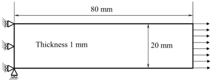
For the Lemaitre damage model, the modeling of the material hardening and the description of the plastic anisotropy are taken the same as in the case of the GTN damage model. In the current contribution, the Lemaitre damage parameters are calibrated using an inverse identification proce-dure along with the experimental uniaxial tensile test for the AA6016-T4 aluminum sheet. This inverse identification strategy is based on least-squares minimization of the difference between the experimental and numerical load–displacement response for a uniaxial tensile test. The geometric dimensions and the boundary conditions for the uniaxial tensile specimen are all specified in Figure 1 (see Kami et al., 2014). The specimen is discretized using the eight-node reduced integration solid finite element (C3D8R) from ABAQUS, with an initial mesh size of 0.5 mm. The identified values of the Lemaitre damage model are summarized in Table 4.
80 mm
20 mm Thickness 1 mm
Figure 1: Geometry and boundary conditions for the uniaxial tensile specimen.
Material β S s Yie
AA6016-T4 12 4.0 1.3 0.0
Table 4: Damage parameters for the Lemaitre damage model.
0 5 10 15 20 25 0
2000 4000 6000
Experiment (from Kami et al., 2015) Lemaitre Damage Model
GTN Damage Model
Fo
rce
(N
)
Displacement (mm)
Figure 2: Tensile load–displacement responses simulated with the GTN and the Lemaitre
damage models, along with the experimental curve taken from Kami et al. (2015).
4 FINITE ELEMENT MODEL
4.1 Nakazima Deep Drawing Test
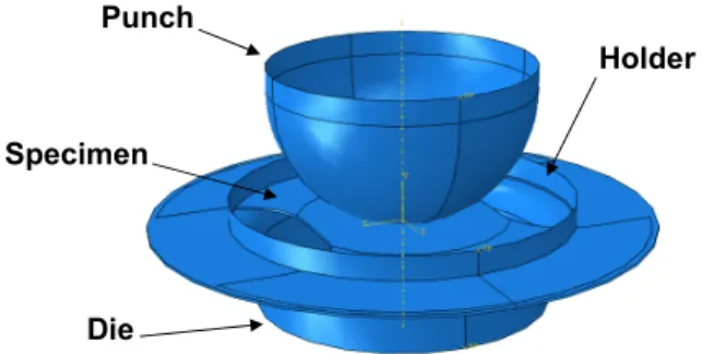
The implemented GTN and Lemaitre damage models, with their associated material parameters, are used in the simulation of the Nakazima deep drawing test (see Figure 3) in order to determine the FLD of the AA6016-T4 aluminum sheet. The geometric parameters for the Nakazima deep drawing process are summarized in Table 5. According to the standard procedure described in ISO 12004-2 (2008), seven specimens with different geometries are considered in the simulations. Each specimen allows for the reproduction of a particular strain path, which is typically encountered in sheet metal forming processes. The general geometry for a given specimen width is illustrated in Figure 4. The seven specimens are designed by varying the width parameter W from 30 mm to 185 mm, which leads to different strain paths in the central part of the specimens, ranging from uniaxial tension to balanced biaxial tension.
Punch
Die Specimen
Holder
Punch diameter 100 mm
Die opening diameter 110 mm
Die profile radius 10 mm
Initial sheet thickness 1 mm
Table 5: Geometric parameters for the Nakazima deep drawing test.
+
+
25 mm R25 mm
W
Figure 4: Specimen geometry and dimensions used in the Nakazima deep drawing test.
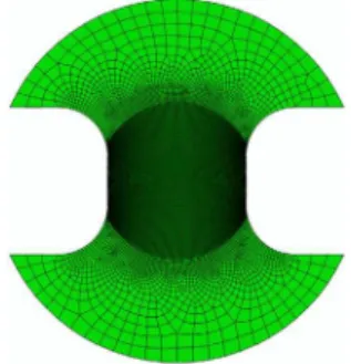
During the Nakazima deep drawing simulation, each specimen is clamped all around its circum-ferential edges so that the material flow is prevented. The Coulomb friction coefficient is taken equal to 0.03 for the contact between the punch and the specimen, while it is taken equal to 0.1 for the contact between the die, the holder and the specimen (see Kami et al., 2015). In addition, a holding force of 100 kN is applied during the forming process. The forming tools are modeled as discrete rigid bodies, while the blank is modeled with the eight-node three-dimensional continuum finite element with reduced integration (C3D8R), which is available in the ABAQUS/Explicit soft-ware. Note that particular attention has been paid to optimizing the mesh of the blank, as illustrat-ed in Figure 5. Indeillustrat-ed, the central part of the blank, which is subjectillustrat-ed to large plastic strains, is discretized with a fine mesh, while the rest of the blank is discretized with a coarse mesh. Moreover, in order to save computational time, the built-in ABAQUS mass scaling technique is used in what follows, with a target time step of 10-6 s and time period of 1 s. These numerical parameters, which lead to reasonable computation times, are selected so that the simulation of the Nakazima deep drawing test is achieved under conditions that are quite similar to those of a quasi-static analysis.
4.2 Mesh Sensitivity Analysis
As already pointed out by several authors in the literature (see, e.g., Tvergaard and Needleman, 1984; Besson et al., 2001; Peerlings et al., 2001), it is nowadays well known that the mesh size has an important influence on the occurrence of strain localization, and particularly for behavior models exhibiting damage-induced softening. In order to analyze the effect of the mesh size on the numeri-cal results, several meshes are used in the simulation of the Nakazima deep drawing test with the specimen of 30 mm width.
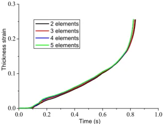
First, the effect of the number of elements in the thickness direction is analyzed by considering, successively, two, three, four and five element layers. Note that for these four different through-thickness FE discretizations, the same in-plane mesh discretization is used, which consists of 0.5×0.5 mm2 in the central part of the specimen. Figures 6 and 7 show the effect of the number of elements in the thickness direction on the evolution of the thickness strain and the punch force– displacement response, respectively. These figures reveal that the number of element layers in the thickness direction has a very small effect on the evolution of the thickness strain, while it has a relatively more noticeable effect on the maximum punch force.
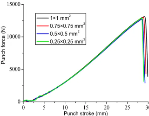
Then, the impact of the in-plane mesh size on the evolution of the thickness strain and the punch force–displacement response is investigated. To this end, the Nakazima deep drawing test is performed again for the specimen of 30 mm width, using four different in-plane meshes for the cen-tral part of the specimen. These in-plane FE discretizations represent coarse, intermediate, fine and very fine meshes, which correspond to mesh sizes of 1×1 mm2, 0.75×0.75 mm2, 0.5×0.5 mm2 and 0.25×0.25 mm2, respectively. Note that, for these four different in-plane mesh discretizations, four element layers in the thickness direction are used. Figures 8 and 9 show the simulated results that are obtained with the four in-plane mesh sizes. Similar to the effect of the number of elements through the thickness, the in-plane mesh size has a small effect on the evolution of the thickness strain, while it has a relatively more perceptible effect on the maximum punch force and on the final punch stroke (i.e., after the sudden load drop).
0.0 0.2 0.4 0.6 0.8 1.0
0.0 0.1 0.2 0.3
Th
ickn
ess
st
ra
in
Time (s) 2 elements 3 elements 4 elements 5 elements
Figure 6: Effect of the number of elements in the thickness direction on the evolution
0 5 10 15 20 25 30 0
5000 10000 15000
Pu
nc
h
fo
rc
e
(N
)
Punch stroke (mm) 2 elements
3 elements 4 elements 5 elements
Figure 7: Effect of the number of elements in the thickness direction on the punch
force-displacement response for the Nakazima test with the specimen of 30 mm width.
In conclusion, the above mesh sensitivity analysis suggests using the fine in-plane mesh (i.e., 0.5×0.5 mm2) with four element layers through the thickness in the remaining simulations of the current study. Indeed, this choice appears as a pragmatic compromise in terms of accurate descrip-tion of the various nonlinear phenomena and reasonable computadescrip-tional times.
0.0 0.2 0.4 0.6 0.8 1.0
0.0 0.1 0.2 0.3
Th
ic
kn
es
s
st
ra
in
Time (s) 1×1 mm2
0.75×0.75 mm2
0.5×0.5 mm2
0.25×0.25 mm2
Figure 8: Effect of the in-plane mesh size on the evolution of the thickness
strain during the Nakazima test with the specimen of 30 mm width.
0 5 10 15 20 25 30
0 5000 10000 15000
Pu
nc
h
fo
rc
e
(N
)
Punch stroke (mm) 1×1 mm2
0.75×0.75 mm2
0.5×0.5 mm2
0.25×0.25 mm2
Figure 9: Effect of the in-plane mesh size on the punch force–displacement
5 LOCALIZED NECKING CRITERIA
In this section, four necking criteria are presented, which will be subsequently used for the predic-tion of strain localizapredic-tion in sheet metals. Three of these criteria are based on the FE analysis of deep drawing process, while the fourth one is based on bifurcation theory. Note that, none of these criteria requires the introduction of additional user-defined parameters, in contrast to the Marciniak and Kuczynski (1967) criterion.
5.1 Criterion of Maximum Second Time Derivative of Thickness Strain
This criterion is based on the analysis of the evolution of thickness strain during the Nakazima deep drawing test. More specifically, the onset of strain localization is associated with the maximum of the thickness strain acceleration, which is obtained by computing the second time derivative of thickness strain in the localized zone (see, e.g., Situ et al., 2006, 2007, 2011; Zhang et al., 2011; Lu-melskyy et al., 2012; Martínez-Donaire et al., 2014). After the maximum in the second time deriva-tive of thickness strain (i.e., thickness strain acceleration) is reached, the localized thinning in the sheet proceeds gradually until the onset of fracture. Based on this numerical criterion, Figure 10 shows an illustration of the onset of localized necking during the simulation of the Nakazima deep drawing test with the specimen of 30 mm width.
0.0 0.2 0.4 0.6 0.8 1.0
-0.02 -0.01 0.00 0.01
2
nd ti
me
d
eri
va
tive
o
f t
hi
ckn
ess
st
ra
in
Time (s) Occurrence of localized necking
Figure 10: Prediction of localized necking based on the maximum of the 2nd time derivative of thickness strain.
5.2 Criterion Based on the Ratio of Equivalent Plastic Strain Increment
localized necking is detected when the ratio of equivalent plastic strain increment in element B to that in element A becomes larger than 10, as illustrated in Figure 11.
0.0 0.2 0.4 0.6
0 10 20 30 40 50
pl
B
/
A
Time (s) Occurrence of localized necking
pl
Figure 11: Prediction of localized necking based on the ratio of equivalent plastic strain increment.
5.3 Maximum Punch Force Criterion
Several theoretical criteria based on the maximum force principle have been developed in the litera-ture for the prediction of diffuse or localized necking in sheet metals (see, e.g., Swift, 1952; Hora et al., 1996; Mattiasson et al., 2006). Based on these earlier contributions, the maximum in the punch force–displacement response during the simulation of the Nakazima test is used here as numerical criterion for the prediction of localized necking (see the illustration in Figure 12).
0 10 20 30
0 5000 10000 15000
Pu
nch
fo
rc
e
(N
)
Punch stroke (mm) Occurrence of localized necking
Figure 12: Prediction of localized necking based on the maximum in the punch force–displacement response.
5.4 Loss of Ellipticity Criterion
theory. This criterion has been established by Rice and co-workers (see, e.g., Rudnicki and Rice, 1975; Stören and Rice, 1975; Rice, 1976) to predict strain localization in the form of an infinite band in a solid otherwise homogeneous. This approach corresponds to the loss of ellipticity (LE) of the partial differential equations governing the associated boundary value problem. The condition of localization, which may be derived from the Hadamard compatibility condition and the static equi-librium equation, is given by the following relation:
det A det n L n 0, (31)
where A denotes the so-called acoustic tensor, n is the normal to the localization band, while L represents the tangent modulus that relates the nominal stress rate tensor to the velocity gradient. The expression of the latter is given by the following relationship (see, e.g., Haddag et al., 2009; Mansouri et al., 2014):
1 2 3
ep
L C L L L , (32)
where Cep is the analytical tangent modulus derived from the constitutive equations, which
corre-sponds to CGTNep for the GTN damage model, and CDM ep
C for the Lemaitre damage model (see Eqs. (17) and (28), respectively). The fourth-order tensors L1, L2 and L3, which only depend on Cau-chy stress components, result from the large strain framework. Their detailed expressions can be found in Haddag et al. (2009).
The loss of ellipticity condition given by Eq. (31) is numerically assessed by computing the de-terminant of the acoustic tensor A for each loading increment. The numerical detection of strain localization is achieved when the minimum of the determinant of the acoustic tensor A, over all possible orientations for the normal n to the localization band, becomes non-positive, as illustrated in Figure 13.
0.0 0.2 0.4 0.6
-2.0x10¹³
0.0
2.0x10¹³
4.0x10¹³
6.0x10¹³
8.0x10¹³
mi
n
de
t(
n
.
L
.
n
)
Logarithmic strain
Occurrence of localized necking
Figure 13: Prediction of localized necking based on the loss of ellipticity criterion.
paths that are typically applied to sheet metals under in-plane biaxial stretching (i.e., ranging from uniaxial tension to balanced biaxial tension).
6 PREDICTION OF FLDS AND COMPARISON WITH EXPERIMENTS
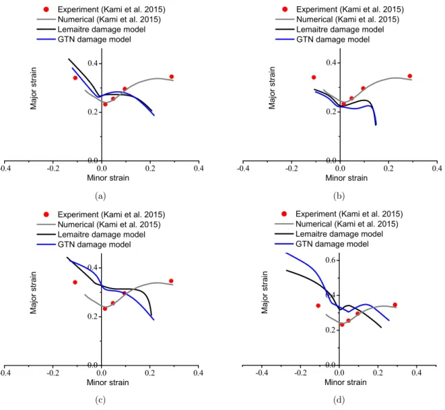
The necking criteria presented in the previous section are combined here with both the GTN and the Lemaitre damage models to predict the FLDs of the AA6016-T4 aluminum sheet. Figure 14 shows a comparison of the FLDs predicted by the four necking criteria, along with the numerical and experimental FLDs provided by Kami et al. (2015). It is worth noting that the numerical FLD given in Kami et al. (2015) is determined on the basis of another specific procedure, which is very different from the numerical methods and criteria adopted in the current work. Indeed, in Kami et al.’s (2015) numerical FLD determination, which closely mimics their experimental FLD determina-tion, the standard specification of the ISO 12004-2 (2008) is followed, where the numerical strain fields and their experimental counterparts are analyzed by the ARAMIS software to determine the numerical and experimental FLDs.
-0.4 -0.2 0.00.0 0.2 0.4 0.2
0.4
Experiment (Kami et al. 2015) Numerical (Kami et al. 2015) Lemaitre damage model GTN damage model
Ma
jo
r st
ra
in
Minor strain -0.4 -0.2 0.0 0.2 0.4
0.0 0.2 0.4
Experiment (Kami et al. 2015) Numerical (Kami et al. 2015) Lemaitre damage model GTN damage model
Ma
jo
r st
ra
in
Minor strain
(a) (b)
-0.4 -0.2 0.00.0 0.2 0.4
0.2 0.4
Experiment (Kami et al. 2015) Numerical (Kami et al. 2015) Lemaitre damage model GTN damage model
Ma
jo
r s
tra
in
Minor strain -0.4 -0.2 0.0 0.2 0.4
0.0 0.2 0.4 0.6
Experiment (Kami et al. 2015) Numerical (Kami et al. 2015) Lemaitre damage model GTN damage model
Ma
jo
r s
tra
in
Minor strain
(c) (d)
Figure 14: Prediction of FLDs using the four localized necking criteria along with the FLDs provided
by Kami et al. (2015): (a) maximum of the 2nd time derivative of thickness strain, (b) ratio of equivalent plastic strain increment, (c) maximum of punch force, and (d) loss of ellipticity.
7 CONCLUSIONS
The Lemaitre damage parameters have been identified using an inverse identification proce-dure based on FE fitting of an experimental load–displacement response of a standard tensile test;
Based on FE simulations of the Nakazima deep drawing test and four different localized neck-ing criteria, numerical FLDs have been determined for the AA6016-T4 aluminum sheet and compared with the experimental FLD. The obtained results suggest that two of the local cri-teria (i.e., those based on the maximum of the 2nd time derivative of thickness strain, and the ratio of equivalent plastic strain increment) yield results that are in good agreement with the experiments in the left-hand side of the FLD and in the neighborhood of the plane-strain ten-sion path, while the global criterion based on the maximum punch force does not seem to be suitable to the prediction of localized necking;
The predictions using the LE criterion provide upper bounds to the classical experimental FLD, which is consistent with the theoretical foundations on which the bifurcation approach is based. On the other hand, this bifurcation approach could be advantageously used to de-sign new materials with improved ductility, by classifying them in terms of formability limits;
The accuracy of the numerically predicted FLDs with respect to experiments may be im-proved by considering various mechanical tests in the identification procedure. Indeed, a number of simple and complex strain paths should be included in the identification procedure in order to provide reliable material parameters, thus improving the accuracy of the predicted FLDs.
References
Abed-Meraim, F., Balan, T., Altmeyer, G. (2014). Investigation and comparative analysis of plastic instability crite-ria: application to forming limit diagrams. International Journal of Advanced Manufacturing Technology 71:1247-1262.
Aravas, N. (1987). On the numerical integration of a class of pressure-dependent plasticity models. International Journal for Numerical Methods in Engineering 24:1395-1416.
Besson, J., Steglich, D., Brocks, W. (2001). Modeling of crack growth in round bars and plane strain specimens. International Journal of Solids and Structures 38:8259-8284.
Brünig, M. (2003). An anisotropic ductile damage model based on irreversible thermodynamics. International Journal of Plasticity 19:1679-1713.
Chaboche, J.L. (1999). Thermodynamically founded CDM models for creep and other conditions: CISM courses and lectures, International Centre for Mechanical Sciences. Creep and Damage in Materials and Structures 399:209-283. Chen, Z., Butcher, C. (2013). Micromechanics modelling of ductile fracture. Solid Mechanics and Its Applications, Springer, Netherlands.
Chu, C., Needleman, A. (1980). Void nucleation effects in biaxially stretched sheets. Journal of Engineering Materi-als and Technology 102:249-256.
Chun, K., Lee, C., Kim, H. (2014). Forming limit criterion for ductile anisotropic sheets as a material property and its deformation path insensitivity, Part II: Boundary value problems. International Journal of Plasticity 58:35-65. Goodwin, G. (1968). Application of strain analysis to sheet metal forming problems in the press shop. SAE Technical Paper No. 680093.
Haddag, B., Abed-Meraim, F., Balan, T. (2009). Strain localization analysis using a large deformation anisotropic elastic–plastic model coupled with damage. International Journal of Plasticity 25:1970-1996.
Hill, R. (1948). A theory of the yielding and plastic flow of anisotropic metals. Proceedings of the Royal Society of London A 193:281-297.
Hill, R. (1952). On discontinuous plastic states, with special reference to localized necking in thin sheets. Journal of the Mechanics and Physics of Solids 1:19-30.
Hora, P., Tong, L., Reissner, J. (1996). A prediction method of ductile sheet metal faillure in FE simulation. Nu-misheet:252-256. Michigan USA.
ISO 12004-2 (2008). International Organization for Standardization, Metallic Materials – Sheet and Strip – Determi-nation of Forming-Limit Curves, Part 2: DetermiDetermi-nation of Forming-Limit Curves in the Laboratory, Switzerland. Kachanov, L.M. (1958). On Creep Rupture Time. Izv. Acad. Nauk SSSR, Otd. Techn. Nauk 8:26-31.
Kami, A., Dariani, B.M., Vanini, A.S., Comsa, D.S., Banabic, D. (2014). Application of a GTN damage model to predict the fracture of metallic sheets subjected to deep-drawing. Proceedings of the Romanian Academy, Series A 15:300-309.
Kami, A., Dariani, B.M., Vanini, A.S., Comsa, D.S., Banabic, D. (2015). Numerical determination of the forming limit curves of anisotropic sheet metals using GTN damage model. Journal of Materials Processing Technology 216:472-483.
Keeler, S., Backofen, W.A. (1963). Plastic instability and fracture in sheets stretched over rigid punches. ASM Transactions Quarterly 56:25-48.
Kojic, M. (2002). Stress integration procedures for inelastic material models within finite element method. ASME Applied Mechanics Reviews 55:389-414.
Lemaitre, J., Chaboche J.L. (1978). Aspect phénoménologique de la rupture par endommagement. Journal de Méca-nique Appliquée 2:317-365.
Lemaitre, J. (1985). A continuous damage mechanics model for ductile fracture. ASME Journal of Engineering Mate-rials and Technology 107:83-89.
Lemaitre, J. (1992). A course on damage mechanics, Springer, Berlin.
Lemaitre, J., Desmorat, R., Sauzay, M. (2000). Anisotropic damage law of evolution. European Journal of Mechanics - A/Solids 19:187-208.
Li, Y.F., Nemat-Nasser, S. (1993). An explicit integration scheme for finite-deformation plasticity in finite-element methods. Finite Elements in Analysis and Design 15:93-102.
Li, J., Li, S., Xie, Z., Wang, W. (2015). Numerical simulation of incremental sheet forming based on GTN damage model. International Journal of Advanced Manufacturing Technology 81:2053-2065.
Lumelskyy, D., Rojek, J., Pecherski, R., Grosman, F., Tkocz, M. (2012). Numerical simulation of formability tests of pre-deformed steel blanks. Archives of Civil and Mechanical Engineering 12:133-141.
Mansouri, L.Z., Chalal, H. and Abed-Meraim, F. (2014). Ductility limit prediction using a GTN damage model cou-pled with localization bifurcation analysis. Mechanics of Materials 76:64-92.
Marciniak, Z., Kuczynski, K. (1967). Limit strains in the process of stretch forming sheet metal. International Jour-nal of Mechanical Sciences 9:609-620.
Martínez-Donaire, A.J., García-Lomas, F.J., Vallellano, C. (2014). New approaches to detect the onset of localised necking in sheets under through-thickness strain gradients. Materials and Design 57:135-145.
Mattiasson, K., Sigvant, M., Larson, M. (2006). Methods for forming limit prediction in ductile metal sheets. In: Santos, A.D., Barata da Rocha, A. (Eds.), Proc. IDDRG’06:1-9, Porto.
Peerlings, R.H.G., Geers, M.G.D., de Borst, R., Brekelmans, W.A.M. (2001). A critical comparison of nonlocal and gradient-enhanced softening continua. International Journal of Solids and Structures 38:7723-7746.
Rice, J.R. (1976). The localization of plastic deformation. Theorical and Applied Mechanics. Koiter ed.:207-227. Rudnicki, J.W., Rice, J.R. (1975). Conditions for the localization of deformation in pressure sensitive dilatant mate-rials. Journal of the Mechanics and Physics of Solids 23:371-394.
Situ, Q., Jain, M.K., Bruhis, M. (2006). A suitable criterion for precise determination of incipient necking in sheet materials. Material Science Forum 519-521:111-116.
Situ, Q., Jain, M.K., Bruhis, M. (2007). Further experimental verification of a proposed localized necking criterion. Proceedings of the Numerical Methods in Industrial Forming Processes - 9th Numiform 907-912.
Situ, Q., Jain, M.K., Bruhis, M., Metzger, D.R. (2011). Determination of forming limit diagrams of sheet materials with a hybrid experimental–numerical approach. International Journal of Mechanical Sciences 53:707-719.
Stören, S., Rice, J.R. (1975). Localized necking in thin sheets. Journal of the Mechanics and Physics of Solids 23:421-441.
Swift, H.W. (1952). Plastic instability under plane stress. Journal of the Mechanics and Physics of Solids 1:1-18. Tvergaard, V. (1981). Influence of voids on shear band instabilities under plane strain conditions. International Journal of Fracture 17:389-407.
Tvergaard, V. (1982a). Ductile fracture by cavity nucleation between larger voids. Journal of the Mechanics and Physics of Solids 30:265-286.
Tvergaard, V. (1982b). Material failure by void coalescence in localized shear bands. International Journal of Solids and Structures 18:659-672.
Tvergaard, V., Needleman, A. (1984). Analysis of the cup-cone fracture in a round tensile bar. Acta Metallurgica 32:157-169.
Yamamoto, H. (1978). Conditions for shear localization in the ductile fracture of void-containing materials. Interna-tional Journal of Fracture 14:347-365.