(Annals of the Brazilian Academy of Sciences) ISSN 0001-3765
www.scielo.br/aabc
Simulated self-organization of death by inherited mutations
JORGE S. SÁ MARTINS1,2, DIETRICH STAUFFER1,3
PAULO M.C. DE OLIVEIRA1,2 and SUZANA MOSS DE OLIVEIRA1,2 1Laboratoire PMMH, École Supérieure de Physique et de Chimie Industrielles
10 rue Vauquelin, F-75231 Paris, France
2Visiting from Instituto de Física, Universidade Federal Fluminense
Av. Litorânea s/n, Boa Viagem, 24210-340 Niterói, RJ, Brasil
3Visiting from Institute for Theoretical Physics, Cologne University, D-50923 Köln, Euroland
Manuscript received on September 26, 2008; accepted for publication on April 1, 2009; contributed byPAULOM.C.DEOLIVEIRA*
ABSTRACT
An agent-based computer simulation of death by inheritable mutations in a changing environment shows a maximal population, or avoids extinction, at some intermediate mutation rate of the individuals. Our results indicate that death seems needed to allow for evolution of the fittest, as required by a changing environment.
Key words:changing environment, computer modeling, evolution, mutation, selection.
INTRODUCTION
More than a century ago, Weissmann argued that aging and death are needed to make place for our children; and children are, in turn, needed to allow for Darwinian evolution through survival of the fittest. Kirkwood (2005) summarized this theory of aging and many other ones, and specific computer models of aging and death were reviewed (Moss de Oliveira et al. 1999, Stauffer et al. 2001, 2006), such as the Penna model (Penna 1995, Moss de Oliveira et al. 1996, Stauffer 2007), and the oldest-old effect (de Oliveira et al. 1998, 1999). A math-ematical argument against immortality was recently given in this sense (de Oliveira 2007a, 2009).
Now we want to understand the need for death through Monte Carlo simulations of individuals. We distinguish between newborns and adults, and take into account environmental changes. They may come from climate change, like ice ages and warmer periods during the existence ofHomo sapiens, or they may be caused by
*Member Academia Brasileira de Ciências Correspondence to: Paulo Murilo Castro de Oliveira E-mail: pmco@if.uff.br
migrations of people from one environment to another. A single environmental change was already used to justify sexual over asexual reproduction (Sá Martins and Moss de Oliveira 1998) or to account for geographic variation (Cebrat and Pekalski 2004). Thus, we may allow the mutation rate of individuals to change in order to find its optimal value. Here “optimal” either means a maxi-mum of the population in a fixed environmental carrying capacity, or survival instead of extinction, depending on which of our two models (A and B) were used.
In these two models, by using sexual reproduction, the genome is represented by two strings ofLbits each, i.e. Lloci. They represent theLmost serious genetic dis-eases. Each mutation damaging the phenotype (i.e. the health of the individual) reduces the survival probability per iteration by a factorx. As genetic load, we count
crossed-over at one randomly selected bit position, the same happening for the mother, and then one of the two resulting bit-strings from the father (the gamete) is com-bined with one of the two from the mother to give the child genome. Mutations are also inherited from the par-ents, andmnew mutations are introduced at birth to each gamete (ifm≥1; form<1, one new mutation is added
with probabilitym). The genetic loadN is the number
of loci (bit positions) where the genome is not adapted (i.e., it is not the same as the ideal string) to the current environment. All the changes in the individuals and the environmental bit-strings are reversible.
Model A’s population is not constant and finds as an optimal m – a mutation rate for which the
equilib-rium population reaches a maximum. Model B follows a tradition of theoretical biology and keeps the population constant except if all adults die out during one iteration; then, we check which mutation rate avoids the extinc-tion of the whole populaextinc-tion. Further details of the two models will be discussed in the corresponding sections.
MODEL A WITH CHANGING POPULATION
In model A, each of the individuals survives the next time step (iteration involving all survivors) with prob-ability xN(1 −P/K), in which P is the current total
population and K is a fixed input parameter, sometimes
called the carrying capacity, representing limitations [due to the lack of food and space] for the population growth. Here,Nis the genetic load, the number of bits that are not
adapted to the current requirement of the environment. The Verhulst factor 1−P/K applies to all individuals,
differently from Sá Martins and Cebrat (2000).
Recessiveness is defined differently in two differ-ent versions A1 and A2 of model A, implying in a dif-ferent computational procedure to determine the genetic load N in each one. For A1, the computational
pro-cedure is to take the logical and of the two bit-strings
of the individual, and then count as N the number of
bit positions where the result of the andoperation
dif-fers from the ideal string. This procedure is close to (Stauffer and Cebrat 2006), and means that heterozy-gous loci do not count for the genetic load N if the ideal string (the environment) has a bit zero in those loci, but count if the bits are set. For A2, we count for
N only those positions where both individual bit-strings
agree with each other (homozygous loci) and disagree with the ideal bit-string. In biological terms, for A1 the allele 0 is always dominant over the recessive allele 1. For A2, in contrast, allele 1 becomes dominant and allele 0 recessive when the environmental bit is 1 instead of 0. Our K is mostly 2 million, the initial population is
K/5, and the resulting equilibrium population is mostly of the order of one million if it does not die out. The two individual bit-strings are mutated independently, each one with a mutation ratem. Each surviving female adult
at each iteration gives birth toB babies, which become
adult at the next iteration; we used B = 4. Mostly 10,000 iterations were made (100,000 for most cases withm < 0.001), and averages were taken from the
second half of this time interval.
CASEA1
Figure 1 shows our main result: the population P has
a maximum as a function ofmat some intermediate m
value. Thus, neither very smallm(“eugenics”) nor very
largem(“instability”) are optimal; an intermediate
mu-tation rate leads to the largestP or the lowesthNi, and, in all cases, to a finite lifespan.
Instead of applying the Verhulst deaths to all ages, Figure 2 shows the correlation betweengeneticdeaths only and genetic load by applying the Verhulst deaths only to the births (Sá Martins and Cebrat 2000). Data are taken from averages calculated at different time steps of a single run for each value ofx.
CASEA2
The modified recessiveness defined above for model A2 reducesN and makes survival possible for a changing environment even for an unrealistically smallx. Forx≥ 0.8 we see in Figure 3 top a plateau for small mutation
ratesm, followed by a decay for a largerm. Thus, there
is no longer the clear population maximum as it was seen in model A1. A similar result was obtained for model A1 in a stable environment (not shown).
MODEL B WITH CONSTANT POPULATION
0.6
0.7
0.8
0.9
1
1.1
1.2
1.3
1.4
0.0001
0.001
0.01
0.1
1
10
p
o
p
u
la
ti
o
n
in
mi
lli
o
n
s
mutation rate
(L,x,p) = (64,.98,.1:+), (64,.98,.01:x); (8,.84,.01:*)
1
10
0.0001
0.001
0.01
0.1
1
10
a
ve
ra
g
e
g
e
n
e
ti
c
lo
a
d
mutation rate
(L,x,p) = (64,.98,.1:+), (64,.98,.01:x); (8,.84,.01:*)
Fig. 1 – Model A1. Search for the optimal mutation rate, in which the population (top) reaches the maximal value and the numberhNiof unadapted loci (genetic load, bottom) gets the minimal, atx=0.98. Forx=0.99,L=64,p=0.01, the results are similar; forx=0.96, the populations
die out for some values of these parameters.
an individual with zero load can still die with a prob-ability 1−x. This selection mechanism may lead to
the extinction of the whole population for some values of the model’s parameters. If there is no extinction at a given time step, the survivors breed, generating new individuals until the initial population size is restored
for the next time step. There is no distinction between males and females, and the population may be regarded as one of hermaphrodites.
0
1
2
3
4
5
6
7
5
10
15
20
25
30
35
40
a
ve
ra
g
e
a
g
e
average genetic load
Verhulst for births only, p = 0.1; x = 0.98(+), 0.99(x)
Fig. 2 – Model A1. Average age of survivorsversusthe number of unadapted loci, when the Verhulst death probability applies to the births only; the individuals are represented by pairs of 64-bit strings and results are shown for various values ofmafter some simulation time. The curves show 1/(|lnx|N).
tions extracted from a uniform distribution in the in-terval[0,2m)is then introduced in this genome, each
one at a random location of a randomly chosen gamete. Thus,m=2 in this model (B) corresponds tom=1 in model A. If M is not an integer, then int(M)mutations
are added, where int(x)is the largest integer contained
in x, and an extra mutation is added with probability
M −int(M). As a result of this strategy,mnew
muta-tions are added to each offspring genome on average. The model treats heterozygous loci in the same way as model A2, that is, they never contribute to the genetic load. A slightly different version of this model, in which x was recalculated at each time step to keep
constant the fraction of deaths, was presented in de Oli-veira (2001) and de OliOli-veira et al. (2008).
The results for this model shown in Figure 4 should be compared to Figure 1. We keep the mutation rate of the environment as p =0.01, the selection strength
as a fixed x = 0.98 and then compute the average
ge-netic loadhNi, the fraction of the population that dies per time step, and the fraction of perfect, or ideal, genomes in the population for different values of the mutation rate m. (Perfect, here, means that no homozygous
un-adapted locus is present, although heterozygous loci can
be present at the individual’s genome). We find that there is an intermediate range of values of the muta-tion rate for which both the genetic load and the death rate go through minima, while the fraction of perfects reaches a maximum. This result matches with what was found, in similar situations, in our model A1. (For
L = 3200 in Fig. 4, extinction happens for mutation rates below 0.1 or above 1.2.).
Our main result refers to the need for a strong se-lection mechanism as a means to enforce a small genetic load: death of the least adapted individuals makes way to fitter ones. In Figure 5 we show the time evolution of the average genetic load of the population for four different sets of parameters. In all four, we simulate a population of 1000 individuals, each one represented by two bit-strings of 3200 bits size, with a mutation rate at birth ofm=1.0. In case (a),x=0.98 (weak selection)
0
0.2
0.4
0.6
0.8
1
1.2
1.4
0.0001
0.001
0.01
0.1
1
10
p
o
p
u
la
ti
o
n
in
mi
lli
o
n
s
mutation rate
Model A2, L=64, p=0.01; x=.98(+), .96(x), .9(*), .8(sq.)
0
2
4
6
8
10
12
14
16
0.0001
0.001
0.01
0.1
1
10
a
ve
ra
g
e
g
e
n
e
ti
c
lo
a
d
mutation rate
Model A2, L=64, p=0.01; x=.98(+), .96(x), .9(*), .8(sq.)
Fig. 3 – Model A2. As Figure 1 but with modified recessiveness and smallerx.
a probability of p = 0.01 at each time step (case (b)),
the average genetic load increases to a value of order 10 and its distribution peaks at a small non-zero value of the same order. Further increase in the rate of envi-ronmental change to p = 0.02 leads the population to
extinction (case (c)). The average genetic load increases rapidly and its distribution widens (Fig. 6). The genetic load accumulates thanks to the joint effects of the
mu-tation rate at birth and a fast environmental change that, even with a weak selection, leads eventually to extinc-tion. The need for a strong selection is now shown: for the same parameters (p andm) but smaller x = 0.95
(case (d)), the population resists and the distribution of genetic load is very similar to the one in case (b).
0.1
1
10
1e-06 1e-05 0.0001 0.001 0.01
0.1
1
10
d
e
a
th
s,
lo
a
d
,
p
e
rf
e
ct
s
mutation rate
64 bits, p=0.01, x=0.98; deaths(+), load(x), perfects(*)
0.001
0.01
0.1
1
10
0
0.2
0.4
0.6
0.8
1
1.2
1.4
d
e
a
th
,
lo
a
d
s,
p
e
rf
e
ct
s
mutation rate
3200 bits, p=.01, x=.95; deaths(+), load(x), perfects(*)
Fig. 4 – Average genetic loadhNi, deaths and number of perfect individuals as a fraction of the population. Top figure for bit-strings of size 64, and bottom figure for 3200. Simulations running for 106time steps.
for larger populations and stronger selection pressure, similar to de Oliveira (2007b).
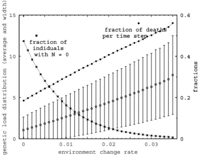
Extinction can then be correlated to features of the distribution of genetic load. It is avoided as long as the average genetic load is not much larger than the width of the distribution. This is more clearly shown
in Figure 7, where we plot the results of simulations of populations with each individual represented by two bit-strings of 2048 bits size, withx = 0.9 (strong
frac-0 50 100 150
0 20 40 60 80 100
a v e r a g e g e n e t i c l o a d < N >
time steps (thousands) a b (line) c (extinction) d (bullets) 0 50 100 150
0 20 40 60 80 100
a v e r a g e g e n e t i c l o a d < N >
time steps (thousands) a b (line) c (extinction) d (bullets) 0 50 100 150
0 20 40 60 80 100
a v e r a g e g e n e t i c l o a d < N >
time steps (thousands) a b (line) c (extinction) d (bullets) 0 50 100 150
0 20 40 60 80 100
a v e r a g e g e n e t i c l o a d < N >
time steps (thousands) a b (line) c (extinction)
d (bullets)
Fig. 5 – Time evolution of average genetic load for the four cases ((a)-(d)) described in the text. Case (c) leads to extinction, while case (d) shows survival when selection is increased.
107
105
103
101
0 50 100 150 200 250 300
f r e q u e n c y
genetic load N a b (line) c (extinction) d (bullets) 107 105 103 101
0 50 100 150 200 250 300
f r e q u e n c y
genetic load N a b (line) c (extinction) d (bullets) 107 105 103 101
0 50 100 150 200 250 300
f r e q u e n c y
genetic load N a b (line) c (extinction) d (bullets) 107 105 103 101
0 50 100 150 200 250 300
f r e q u e n c y
genetic load N a
b (line)
c (extinction)
d (bullets)
Fig. 6 – Distribution of genetic load for the four cases ((a)-(d)) de-scribed in the text.
tion of individuals with zero load decreases. Beyond
p=0.35, this fraction vanishes and extinction is the
out-come of the simulation. In the same plot, we also show the fraction of individuals that die (for genetic reasons only, in this model) at each time step. As p increases,
survival of the population becomes more difficult and causes this fraction to be ever increasing.
CONCLUSION
In all our models, the genetic heritage of a diploid in-dividual is represented by a pair of bit-strings, which undergo mutations at birth, while the ideal phenotype is mapped into a single bit-string. Environmental change is translated into a mutation of this ideal phenotype. The genetic load of an individual is determined by a
com-0 5 10 15
0 0.01 0.02 0.03
g e n e t i c l o a d d i s t r i b u t i o n ( a v e r a g e a n d w i d t h )
environment change rate
0 0.2 0.4 0.6 f r a c t i o n s fraction of indiduals
with N = 0
fraction of deaths per time step
0 0.2 0.4 0.6 f r a c t i o n s fraction of indiduals
with N = 0
fraction of deaths per time step
Fig. 7 – Average genetic load – open circles – and width of the dis-tribution of load – error bars – (y scale on the left), fraction of the population with no genetic load and fraction of deaths per time step (y scale on the right). Values correspond to averages taken after 5000 initial time steps, up to 106. Similar results are obtained forL≤32768.
parison between its genetic strings and the ideal pheno-type. This genetic load determines the death probability of each individual.
Our results come from simulations with a fixed rate of environmental change and a fixed value for the parameter that measures selection strengthx. We show
that population fitness, determined by its size, reaches a broad maximum, while the average genetic load reaches a minimum, for some intermediate range of the mutation rate at birth (model A1). So, nature has self-organized its cellular error correction machinery to ensure a mutation rate within some range.
On the other hand, when the rate of environmen-tal change increases, our results are consistent with the interpretation that selection has to get stronger to avoid population extinction (model B).
A more realistic approach would assign a different selective value for each different bit position, since dif-ferent inherited diseases differ in their danger to survival. However, since these values would have to be free pa-rameters, their introduction in the model would render it almost useless.
ACKNOWLEDGMENTS
RESUMO
Simulação computacional de agentes individuais que se repro-duzem e morrem por acúmulo de mutações herdadas mostra um máximo da população ou evita extinção, para taxas de mu-tação intermediárias. Assim, as mortes parecem necessárias para a evolução dos mais adaptados a um ambiente mutante.
Palavras-chave: ambiente mutante, evolução, modelagem
computacional, mutação, seleção.
REFERENCES
CEBRATSANDPEKALSKIA. 2004. The Role of Dominant Mutations in the Population Expansion. Lect Notes Comp Sci 3039: 765–770.
DEOLIVEIRAPMC. 2001. Why Do Evolutionary Systems
Stick to the Edge of Chaos? Theory Biosc 120: 1–19. DEOLIVEIRAPMC. 2007a. A Importância das Flutuações
em Biologia. Rev bras ens fis 29: 377–384.
DEOLIVEIRAPMC. 2007b. Chromosome Length Scaling in Haploid, Asexual Reproduction. J Phys CM19, 065147, 9 p.
DEOLIVEIRA PMC. 2009. Why Must We All Die? The Combined Role of Dissipation and Fluctuations in Evolu-tionary Biology. In: HIRTREITERCANDSCHNEIDERJJ
(Eds), Lectures on Socio- and Econo-Physics, Springer-Verlag, Heidelberg.
DEOLIVEIRAPMC, MOSS DEOLIVEIRAS, BERNARDES
AT ANDSTAUFFERD. 1998. Siblings of Centenarians Live Longer: a Computer Simulation. The Lancet 352: 911–911.
DEOLIVEIRAPMC, MOSS DEOLIVEIRAS, BERNARDES
ATANDSTAUFFERD. 1999. Monte Carlo Simulations of Inherited Longevity. Physica A262: 242–248.
DEOLIVEIRAPMC, MOSS DEOLIVEIRAS, STAUFFERD, CEBRATSANDPEKALSKIA. 2008. Does Sex Induce a Phase Transition? Eur Phys J B 63: 245–254.
KIRKWOODTBL. 2005. Understanding the Odd Science of Aging. Cell 120: 437–447.
MOSS DE OLIVEIRA S,DE OLIVEIRAPMCANDSTAUF
-FERD. 1996. Ageing with Sexual and Asexual Reproduc-tion: Monte Carlo Simulations of Mutation Accumulation. Braz J Phys 26: 626–630.
MOSS DE OLIVEIRA S,DE OLIVEIRAPMCANDSTAUF -FER D. 1999. Evolution, Money, War and Computers. Teubner, Leibzig-Stuttgart.
PENNATJP. 1995. A Bit-String Model for Biological Aging. J Stat Phys 78: 1629–1633.
SÁMARTINSJSANDCEBRATS. 2000. Random Deaths in a Computational Model for Age-Structured Populations. Theory Biosc 119: 156–165.
SÁMARTINSJS ANDMOSS DEOLIVEIRAS. 1998. Why Sex: Monte Carlo Simulation of Survival After Catastro-phes. Int J Mod Phys C 9: 421–432.
STAUFFER D. 2007. The Penna Model of Biological
Ag-ing. Bioinformatics and Biological Insights 1: 91–100 (www.la-press.com/article.php?article_id=520).
STAUFFERDANDCEBRATS. 2006. Extinction in Genetic Bit-String Model with Sexual Reproduction. Adv Compl Syst 9: 147–156.
STAUFFER D, DE OLIVEIRA PMC, MOSS DE OLIVEIRA
S, PENNATJPANDSÁMARTINSJS. 2001. Computer Simulations for Biological Asexual and Sexual Reproduc-tion. An Acad Bras Cienc 73: 15–32.