CREEP ANALYSIS OF STEEL-CONCRETE COMPOSITE BEAMS USING GENERALIZED BEAM THEORY

In Figure 2 the two areas labeled Nabarro-Herring creep 16,17 and Coble creep 18 are based on the theoretical relationships developed for diffusional creep, the area labeled

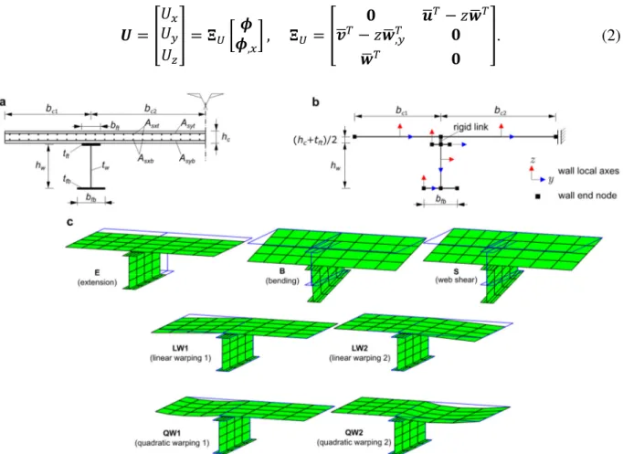
The purpose of this work is to present a three-dimensional beam element for the structural and thermal analysis of reinforced concrete, steel and composite steel and

Posteriormente, no Capítulo IV, é abordado o que constitui o objeto central do trabalho, infere-se da importância do SGI recorrendo, para o efeito, à análise de

first obtained the creep deformation in a large-span reinforced concrete beam, then steel beam-column connections, and lastly the deformations in a pedestrian bridge using

Dynamic mechanical analysis and creep - by using Findley and Burger's methods - tests were performed aiming to evaluate the viscoelastic properties of the composites, in

(2006) studied through a FE formulation the behavior of steel-concrete composite beams under long- term loads, including simultaneously the effect of concrete creep, shrinkage

A computationally efficient GBT-based beam finite element for calculating buckling (bifurcation) loads of steel-concrete composite beams was proposed, which accounts for shear

4.3.5 Composite model for the characterization of the long-term properties 137 4.3.6 Prediction of dam concrete creep strains under compression based on experimental tests

REFERENCES

[1] Schardt R., “Eine erweiterung der technischen biegetheorie zur berechnung prismatischer faltwerke”, Stahlbau, 35, 161-171, 1966 (German).
[2] Schardt R., Verallgemeinerte Technische Biegetheorie, Springer Verlag, Berlin, 1989 (German).
[3] Camotim D., Basaglia C., Bebiano R., Gonçalves R., Silvestre N., “Latest developments in the GBT analysis of thin-walled steel structures”, Proceedings of Int. Colloquium on Stability and Ductility of Steel Structures, E. Batista et al. (eds.), Rio de Janeiro, Brazil, 33-58, 2010.
[4] Camotim D., Basaglia C., Silva N., Silvestre N., “Numerical analysis of thin-walled structures using Generalised Beam Theory (GBT): Recent and future developments”, Computational Technology Reviews, B. Topping et al. (eds.), Saxe-Coburg, Stirlingshire, 315-354, 2010.
[5] Camotim D., Basaglia C., “Buckling analysis of thin-walled steel structures using Generalized Beam Theory (GBT): state-of-the-art report”, Steel Construction, 6(2), 117-131, 2013.
[6] Gonçalves R., Camotim D. “Steel-concrete composite bridge analysis using Generalised Beam Theory”, Steel and Composite Structures, 10(3), 223-43, 2010.
[7] Henriques D., Gonçalves R., Camotim D. “A physically non-linear GBT-based finite element for steel and steel-concrete beams including shear lag effects”, Thin-Walled Structures, 90, 202-215, 2015.
[8] Henriques D., Gonçalves R., Camotim D. “GBT-based finite element to assess the buckling behavior of steel-concrete composite beams”, Thin-Walled Structures, 107, 207-220, 2016. [9] EN1994-1-1:2004, Eurocode 4: Design of Composite Steel and Concrete Structures. Part 1-1:
General Rules and Rules for Buildings, CEN, Brussels, Belgium, 2004.
[10] Bažant Z., Wu S. “Dirichlet series creep function for aging of concrete”, Journal of the Engineering Mechanics Division, 9(2), 367-387, 1973.
[11] Ranzi G., Leoni G., Zandonini R., “State of the art on the time-dependent behaviour of composite steel-concrete structures”, Journal of Constructional Steel Research, 80, 252-263, 2013.
[12] Gara F., Leoni G., Dezi L., “A beam finite element including shear lag effect for time-dependent analysis of steel-concrete composite decks”, Engineering Structures, 31, 1888-902, 2009.
(10)
[14] Gonçalves R., Ritto-Corrêa M., Camotim D., “A new approach to the calculation of cross-section deformation modes in the framework of Generalized Beam Theory”, Computational Mechanics,
46(5), 759-781, 2010.
[15] Gonçalves R., Camotim D., “Geometrically non-linear Generalised Beam Theory for elastoplastic thin-walled metal members”, Thin-Walled Structures, 51, 121-129, 2012.
[16] MATLAB, version 7.10.0 (R2010a), The MathWorks Inc., Massachusetts, 2010.
[17] Bathe K. J., ADINA System, ADINA R&D Inc., 2017.
Imagem
Figure 1: Steel-concrete composite beam (a) cross-section geometry, (b) wall mid-lines and boundary  conditions, and (c) cross-section deformation modes