Finite element study of effective width in steel-concrete composite beams under long-term service loads

(1)

Finite element study of effective width in steel-concrete composite

beams under long-term service loads

Abstract

In this work, a finite element-based approach is presented to study the ef-fective width variation in non-pre-stressed steel-concrete beams under the serviceability stage, including time dependent effects such as concrete creep, shrinkage and cracking. For this purpose, the viscoelasticity theory in conjunction with a nonlinear cracking monitoring algorithm is used to trace the nonlinear viscoelastic response of the structure along time. The present numerical model is fully three-dimensional and permits the inclu-sion of partial interaction at the slab-beam interface. A comprehensive study is carried out on the long-term response of a composite girder bridge previously studied by other researches. Then, previous results are revised and extended herein. Potential shortcomings of some standard codes relat-ed to the effective width evaluation are also investigatrelat-ed. It is demonstrat-ed that the slab effective width varies sharply along the beam axis in the short-term, while it approaches to the actual slab width in the long-term. For the studied example, the common assumption of using only the middle layer of the reinforced concrete (RC) slab for the effective width calculation is revised with a through-thickness integration procedure. The influence of some creep and shrinkage models as well as the ultimate tensile concrete strain on the effective width response is also assessed. Finally, a simple formula is proposed to evaluate the short-term slab effective width for the studied example.

Keywords

Effective width, steel-concrete composite beams, finite element, reinforced concrete.

1 INTRODUCTION

The use of steel-concrete composite beams has a major role in building and bridge engineering. In recogni-tion to this, design guidelines are provided in most regularecogni-tions around the world, where the concept of effective width is introduced in order to avoid complex calculations. The actual non-uniform stress distribution acting across a slab width due to the shear lag effect, with a maximum stress value occurring at the RC slab edge or cen-ter, is addressed using an equivalent uniform stress distribution. This distribution acts across a namely reduced effective width with a stress value equating the maximum value of the actual stress distribution. This simplifica-tion allows engineers to use elementary beam theory for calculating stresses and deflecsimplifica-tions under short-term and long-term loads without loss of accuracy. Nevertheless, expressions for the effective width evaluation as pre-sented in various design specifications could not consider the potential variability of such quantity due to con-crete rheology. In fact, within the specialized literature, there are various experimental and finite element (FE) studies that focus on the slab effective width under other effects such as different load intensities (ultimate and

Lucas H. Reginatoa_* Jorge L. P. Tamayob Inácio B. Morschc

a _{Centro de Mecânica Aplicada e Computacional}

(CEMACOM), Escola de Engenharia, Universida-de FeUniversida-deral do Rio GranUniversida-de do Sul (UFRGS), Porto Alegre, RS, Brazil. E-mail:

lucasregi-nat@hotmail.com

b _{Departamento de Engenharia Civil, Escola de}

Engenharia, Universidade Federal do Rio Grande do Sul (UFRGS), Porto Alegre, RS, Brazil. E-mail: jorge.tamayo@ufrgs.br

c _{Departamento de Engenharia Civil, Escola de}

Engenharia, Universidade Federal do Rio Grande do Sul (UFRGS), Porto Alegre, RS, Brazil, E-mail: morsch@ufrgs.br

*Corresponding author

http://dx.doi.org/10.1590/1679-78254599

(2)

rini et al. (2006) studied through a FE formulation the behavior of steel-concrete composite beams under long-term loads, including simultaneously the effect of concrete creep, shrinkage and cracking of the RC slab in the FE analysis, emphasis was given to the effective width evaluation along time. Chen and Zhang (2006) analyzed the effect of external pre-stressing on the slab effective width in simply supported steel-concrete beams. Dezi et al. (2006) studied the effective width in pre-stressed twin-girder in composite beams by considering only the creep effect. Castro et al. (2007) verified the suitability of the effective width provided for some standard codes consid-ering the elastic and elastic-plastic behavior of materials using the FE method. In Nie et al. (2008), a definition of the effective width is presented for ultimate load analysis of composite beams under sagging bending moments. Xue et al. (2008) investigated the combined effect of creep and shrinkage and relaxation of pre-stressing tendons on the long-term response of simply supported steel-concrete composite beams. Gara et al. (2009) proposed a new beam finite element to take into account the shear lag effect and time effects due to concrete creep in compo-site beams.

Salama and Nassif (2011) tested eight simply supported steel-concrete specimens and proposed an effective width formula for steel-concrete composite beams under short-term loads. Nie and Tao (2012) calculated ulti-mate bending moments using simplified design formulas for the slab effective width. In Zhu et al. (2015), a pre-diction formula for the effective width evaluation of I-girder, twin I-girder and box-girder under short-term loads was proposed. Galuppi and Carfagni (2016) used the strain energy functional to determine a slab effective width considering the nonlinear behavior of connectors. Otherwise, Yuan et al. (2016) stated that the evaluation of the effective width should be based on the element response rather than the value in a section. Then, two theoretical models were proposed for studying the slipping at the slab-beam interface and the shear lag effect. Recently, Zhu et al. (2017) studied the shear-lag effect in composite twin-girder decks by means of an analytical approach and proposed a new definition for the effective width based on positive and negative shear-lag patterns along the beam axis.

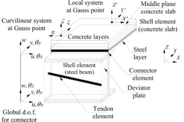
As a practical matter, only a few studies (Macorini et al., 2006, Chen and Zhang 2006, Xue et al. 2008) have addressed the effect of concrete creep, shrinkage and cracking simultaneously over the entire service life of non-pre-stressed steel-concrete composite beams with emphasis to the effective width evaluation. In this work, Maco-rini et al.’s girder bridge is studied and their numerical results are verified. Potential short-comings of some cur-rent design specifications are also commented for the studied example. For this purpose, an in-house FE program namely VIMIS developed by the authors is used for the numerical simulations. The used FE model is able to cap-ture properly the nonlinear response due to concrete cracking and the viscoelastic response of the RC slab. The shear lag effect is included intrinsically in the model since the RC slab is modeled three-dimensionally. In Figure 1 is illustrated a typical portion of a steel-concrete composite beam as modeled in VIMIS (e.g. Tamayo et al. 2013, Tamayo et al. 2015, Tamayo and Awruch, 2016, Moscoso et al. 2017, Dias et al. 2015). In this manner, the contri-bution of the present work can be summarized as follow: 1) Verification of Macorini et al.’s results with the pre-sent FE model in view of the lack of more results about the variation of the effective width along time; 2) Compar-ison of computed FE effective width ratios with some regulations (e.g. AASHTO 2012; NBR8800, 2008; EC4, 2005; GB50017, 2003) and researches formulas (e.g. Yuan et al. 2016, Gara et al. 2009 and Zhu et al. 2017); 3) Suitabil-ity of the effective width calculation based on the RC slab middle layer stresses versus a through-thickness inte-gration procedure; and 4) Study of the effect of some creep and shrinkage models such as ACI Committee 209 (1992), B3 (Bazant and Baweja 1995), GL (Gadner and Lockman 2001), CEB MC 90 (CEB 1993), CEB MC 99 (CEB 1999) and FIB MC 2010 (FIB 2010) as well as the ultimate tensile concrete strain on the effective width response. Finally, a simplified expression is proposed for the short-term effective width evaluation for the studied example.

(3)

2 CONSTITUTIVE MODELS

2.1 Steel beam and shear stud connections

The state of stress in the steel beam is modeled using the von Mises elasto-plastic law with linear hardening. The stud shear connectors, which are represented by special beam-column elements, follow a nonlinear shear force-slip curve since the beginning of loading along the longitudinal and transversal directions of the composite beam, while full compatibility is assumed in other directions. Both the steel beam and the shear connectors do not present rheological behavior and remain practically elastic within the serviceability stage.

2.2 Reinforced concrete slab

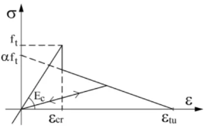
Concrete in compression is modeled by using an elasto-plastic law following a modified Drucker-Prager yield criterion with nonlinear hardening. The response of concrete under tensile stresses is assumed to be linear elastic until the tensile strength ft is reached, and then an orthotropic behaviour is considered. Cracks are assumed to occur in planes perpendicular to the direction of the maximum tensile stress as soon as this stress reaches the tensile strength. A strain-softening law is used for the tensile nonlinear behaviour to take into consideration the tension stiffening effect. In this work the linear descending stress-strain law shown in Figure 2 is adopted. This function is limited on one end by the cracking strain (εcr=ft/Ec), where Ec is the elastic Young’s modulus, and with the ultimate tensile strain εtu on the other end. This last strain is usually approximated by εtu≈(10-20).εcr for RC slabs. However, a value of 0.1 has been suggested in other references (e.g. Liang et al. 2005, Baskar et al. 2002 and Rex and Easterling, 2000) for RC slabs in composite sections. The model also considers the opening and closing of cracks due to concrete stress redistribution along time.

Concrete creep and shrinkage are included in the analysis using the viscoelasticity theory, which is linked to the nonlinear behaviour of cracked concrete. The concrete is considered an aging viscoelastic material both in tension and compression. The viscoelastic behaviour is expressed in terms of an integral form namely Volterra’s integral equation using a relaxation function so as to account for creep deformation. The Volterra’s integral equa-tion is solved using the Kelvin’s chain model, where the relaxaequa-tion funcequa-tion is expanded in a series of exponential terms. Only mechanical strains are considered to enter in the short-term concrete constitutive model. The reader is referred to the works of Macorini et al. (2006) and Dias et al. (2015) for a complete description of the algo-rithm.

Figure 2: Softening law for cracked concrete.

3 FINITE ELEMENT MODELS

3.1 Concrete slab

(4)

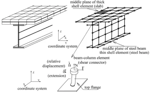
two-node beam-column elements, which join one node from the middle plane of the RC slab with the correspond-ing node of the upper steel flange as shown Figure 4. These bar elements are located at the real positions of the shear connectors along the longitudinal axis of the beam.

(a) Layered thick shell finite element for RC slab. (b) Thin-shell element for steel beam. Figure 3: Finite elements.

Figure 4: Shear connectors.

4 EFFECTIVE WIDTH EVALUATION

Two approaches are used for calculating the effective width in this work. Firstly, the effective width can be calculated considering only the middle layer stress distribution of the RC slab (Macorini et al. 2006), as shown in Figure 5, with the following equation:

 





 



2

2 max

1

b

b x y

x

ef

dy

b



(1)

where bef and b are the effective width and slab width, respectively, and σx is the normal stress acting across the

(5)

completely cracked regions (e.g. hogging bending moment regions), the reinforcing bars are responsible for resisting external stresses. Hence, the effective width value is evaluated according to Eq. 3.

 



    



₂ 2 max 2 2 t t y x b b x ef

dy

b



(2)

 



  



2 2 max

1

b b r y r ef

dy

b



(3)

where σr and σr,max denote, respectively, the average stress measured in the top and the bottom bars at a given

location y along the concrete width, and the maximum value of this quantity along the slab width (Macorini et al., 2006). In this work, all results are expressed in terms of the effective width ratio, which is intrinsically defined as

η=bef/b.

Figure 5: Geometry for the effective width evaluation.

5 APPLICATION

5.1 Interior span of Girder Bridge under long-term loading (Macorini et al. 2006)

(6)

mod-therefore boundary conditions are not necessary the same at the fixed ends; 2) Macorini et al.’s model uses a spe-cial connection system with zero-length contact elements located at the slab-beam interface for simulating slip-ping, meanwhile a special beam-column element is used in the present FE model; 3) Out-plane shear stresses are considered elastic in Macorini et al.’s concrete model at all times, whereas they are viscoelastic in this work; 4) The manner in which cracked strains are treated in each constitutive model is different. Also, the ultimate tensile strain εtu is not reported in the quoted reference, and then a value of 0.1 is used herein, unless otherwise stated. Results of Macorini et al.’s program namely ADAPTIC (or ADAP.) are plotted for comparison whenever they are available.

Figure 6: Geometry of cross-section.

Figure 7: Finite element mesh and boundary conditions at the fixed ends.

Table 1: Material properties.

Concrete

Young’s-Modulus E28 30000 MPa

Compressive-Strength fck 35 MPa

Tensile-Strength ft 3.05 MPa

Ultimate Compressive Strain εu(-) 2.5 %

Ultimate Tensile Strain εu(+) 1.0 %

Poisson’s Ratio υ 0.15

Structural steel

Yield-Stress fy 250 MPa

Poisson’s Ratio υ 0.30

Reinforcing steel

Yield-Stress fy 250 MPa

Ultimate-Stress fu 350 MPa

Connectors

Lateral-Stiffness Kx 1.50 E+04 kN/cm

(7)

5.1.1 Linear viscoelastic analysis

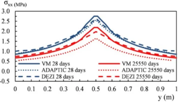
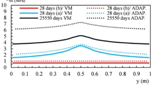
Firstly a viscoelastic analysis without considering the effect of concrete shrinkage and cracking is carried out. An external uniformly distributed load 100 kN/m is applied at 28 days after concrete casting and the computed results were monitored for 70 years (25550 days). The present FE results, namely VM in the figures, are depicted in Figure 8. Figures 8(a)-(b) show the longitudinal normal stress distribution across the slab width for the middle layer of the RC slab at the mid-span and fixed end, respectively, and for two time instants (28 and 25550 days). As it may be observed, good agreement is found between present and Macorini et al.’s results. Concrete creep only shifts the stress distributions to lower values (i.e. absolute values) after 70 years, while maintaining the same bell-shaped form of the distributions. As a result, Figure 8(c) shows that the effective width ratio η remains con-stant in time. Maximum concrete stress evolutions are shown in Figure 8(d). The calculation of the effective width according to some standard codes is associated to the definition of an equivalent span length Le, which can be considered equal to 0.7L2 and 0.25(L1+L2) for sagging and hogging bending moment regions, respectively, whereas L1 denotes the side length and L2 is the mid-span length. For the present continuous composite girder L1=L2=25 m.

Due to symmetry considerations, in Figures 8(e)-(f) are depicted the η values along half of the normalized beam axis x/L at all times, where x and L represent the current coordinate position and beam span length, respec-tively. In Figure 8(e), the computed η values are compared with those obtained using the ASSHTO (2012), NBR8800 (2008), EC4 (2005) and GB50017 (2003) regulations, meanwhile in Figure 8(f), they are compared with other approaches based on the works of Zhu et al. (2015), Yuan et al. (2016) and Gara et al. (2009). As it may be observed, the η values are almost constant in time although they present a quite irregular profile along the beam axis. The predicted values obtained with the EC4 (2005) and NBR8800 (2008) regulations acceptably match the current FE results at the mid-span and fixed ends only. Meanwhile, the ASSHTO (2012) code predicts a constant value 1.0 at all times. Differently from the aforementioned regulations, the Chinese code GB50017 (2003) uses a coupled criterion for η, which includes the use of the beam span length and slab thickness. When the slab thickness is excluded from the criterion (e.g. namely GB50017 w/o th. curve in Figure 8(e)), the calculat-ed η values conduct to a similar pattern as obtained for the EC4 (2005) code. Otherwise, when the complete crite-rion is used (e.g. GB50017 w/th. curve), a constant lower limit value 0.5 is obtained. This last value could be ex-cessively conservative at some beam locations.

(8)

(a) Stress distribution in the middle layer of RC slab

at the mid-span. (b) Stress distribution in the middle layer of RC slab at the fixed end.

(c) Effective width ratio variation with time. (d) Maximum concrete stress variation with time in the middle layer at mid-span and fixed end.

(e) Comparison of effective width ratio

along the beam axis with standard codes.

(f) Comparison of effective width ratio

along the beam axis with researcher’s formulas.

(g) Effective width ratio in terms of width/span

(9)

5.1.2 Linear viscoelastic analysis with shrinkage

In this part of the study, the concrete shrinkage effect is included in the analysis one day after concrete cast-ing. In fact, this time corresponds to the start of the time-history analysis in the FE model. Figures 9(a)-(b) show the longitudinal normal stress distribution across the slab width at the mid-span and fixed end, respectively, for the middle layer of the RC slab and for two time instants (28 and 25550 days). As it may be observed, acceptable matching is found between present and Macorini et al.’s results for the short-term, but some differences are re-ported for the long-term response. Firstly, concrete shrinkage acts alone producing a uniform stress distribution (28 days (b)/VM curve). Secondly, a uniform load is suddenly applied at 28 days, yielding negative and positive shear-lag patterns at the mid-span and fixed end, respectively (see 28 days (a)/VM curves). At the end, higher and smoother stress values are obtained at the long-term. Precisely, in Figure 9(c) is depicted the variation of η with time. As it may be observed, η approaches to 1.0 since the beginning of the analysis when concrete shrinkage acts alone. Then, the η value is suddenly reduced at both cross sections immediately after loading is applied (0.5 and 0.63 for the mid-span and fixed end, respectively). This reduction occurs because the applied load modifies the stress distributions, concentrating higher stress at the slab-beam intersection and slab edges. Finally, η reaches values of 0.95 and 0.80 at mid-span and fixed end at the long-term, respectively. Maximum concrete stress evolu-tions are depicted in Figure 9(d).

Figures 9(e)-(f) compare the η variations in space and time obtained with the present FE model and other methodologies. As it can be seen, the FE effective width ratios obtained at 28 and 25550 days are quite dissimilar although with the latter approaching to 1.0 along the beam axis, with exception of the region near the fixed end (0<x/L< 0.15). In relation to code regulations, the η values predicted by the ASSTHO (2012) and GB50017 (2003) (i.e. GB50017 w/o th. curve) specifications match well the long-term response. Otherwise, the EC4 (2005) and NBR 8800 (2008) code predictions are on the unsafe side in the central region of the beam (0.35<x/L<0.5) for the short-term, but they are conservative for the long-term. The curve namely GB50017 w/th. in Figure 9(e), which includes the slab thickness criterion, can be interpreted as a lower limit. In Figure 9(f), Gara et al.’s and Yuan et al.’s method are adequate for the long-term response, whereas Zhu et al.’s approach is on the unsafe side in the central region of the beam for the short-term.

(10)

(c) Effective width ratio variation with time. (d) Maximum concrete stress variation with time in _{the middle layer at mid-span and fixed end.}

(11)

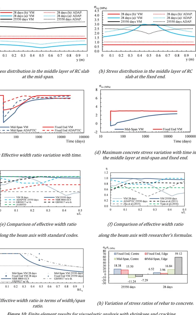
5.1.3 Non-linear viscoelastic analysis with shrinkage and cracking

A more realistic study is carried out including all the aforementioned effects plus concrete cracking. Concrete stress distributions across the slab width at the mid-span and fixed end for the middle layer of the RC slab are shown in Figures 10(a)-(b), respectively. As it may be observed in Figure 10(a), acceptable matching is found between present and Macorini et al.’s results at all times at the mid-span section. Otherwise, it is noticed that con-crete stresses near the slab center at the fixed end in Figure 10(b) reach the concon-crete tensile strength immediate-ly after loading is applied (see 28 days (a)/VM curve). Once cracks are initiated at the slab center, tensile stresses redistribute to the uncracked regions (edges) and the slab effective width reaches the actual slab width, yielding a uniform stress distribution at 25550 days. These long-term stresses are slightly lower than the specified concrete tensile strength (3.05 MPa), indicating that concrete between cracks is still able to resist external stresses. This last fact is not expected in current design practice, since hogging moment regions are considered to be completely cracked. Maybe, the ultimate tensile strain value εtu used in the softening law for cracked concrete could influence this final stress distribution. This point will be investigated in section 5.1.6.

The η values and maximum stress concrete evolutions are depicted in Figures 10(c)-(d), respectively. The η

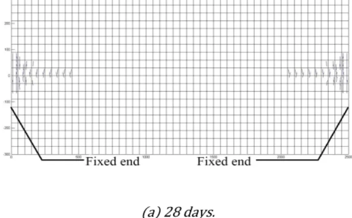
evolution along the beam axis is presented in Figures 10(e)-(f). The values presented in these figures are quite similar to those obtained for the viscoelastic analysis with shrinkage, then similar conclusions can be inferred although it should be highlighted that concrete cracking contributes with higher short-term effective width ratios at the fixed end. In Figures 10(g)-(h), the η value versus various width/span ratios and stress ratios of rebar to concrete are plotted, respectively. As in the previous analysis, the same trend is also observed. However, the fixed end η value at 25550 days is now above the curve predicted by Chinese regulation which excludes the thickness criterion (GB50017w/o th.). In Figure 11 are shown the cracking patterns for the middle layer of the RC slab at 28 and 25550 days.

In Figure 12 are shown the results related to the longitudinal stresses and effective width ratios for the rein-forcing bars. Present and Macorini et al.’s results were calculated considering the average stress values of the top and bottom reinforcing longitudinal bars. Figures 12(a)-(b) display the normal stress distributions across the slab width for the mid-span and fixed end, respectively. As it may be observed, present and Macorini et al.’s results match well for the short-term values (e.g. 28 days (b)/VM and 28 days (a)/VM curves), but they disagree at the long-term. Mainly, the stress distribution is particularly different at the fixed end, where a constant uniform stress increment with time is observed for the present model, meanwhile Macorini et al.’s results showed a non-uniform stress profile. Nevertheless, the average stress value of Macorini et al.’s distribution approximately matches the long-term stress value predicted here. Also, the η variation with time shown in Figure 12(c), acceptably match Macorini et al.’s results since the beginning of the analysis, but they start to diverge after 100 days at the fixed end. This divergence is due to the stress profiles already depicted in Figure 12(b). The η profile shown in Figure 12(d) is quite irregular along the beam axis, approaching to 1.0 at x/L = 0 and x/L = 0.5 for 25550 days. The EC4 and NBR 8800 regulations only match the short-term η values at the fixed end and mid-span.

(12)

(c) Effective width ratio variation with time. (d) Maximum concrete stress variation with time in _{the middle layer at mid-span and fixed end.}

(13)

(a) 28 days.

(b) 25550 days.

Figure 11: Cracking patterns for viscoelastic analysis with shrinkage and cracking.

(a) Averaged stress distribution on top and bottom

(14)

5.1.4 Effective width evaluation considering slab thickness integration

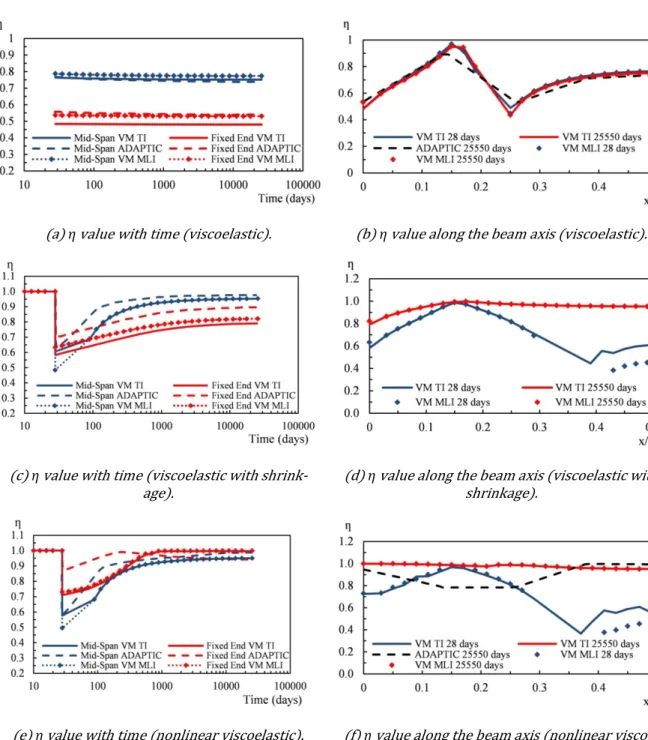
In previous sections, the effective width ratio η was evaluated according to the actual stress distribution across the slab width at the middle layer of the RC slab, namely here Middle Layer Integration (MLI) approach (see Equation (1)). To validate this assumption, the effective width ratio was also calculated considering the actu-al stress distribution actu-along the slab thickness, namely here Totactu-al Integration (TI) approach, according to Equation (2). As it is well-known, concrete stresses vary along the slab thickness and across the slab width under flexure. In Figures 13(a)-(b) are shown the η variations with time and along the beam axis, respectively, for the viscoelastic analysis.

(a) η value with time (viscoelastic). (b) η value along the beam axis (viscoelastic).

(c) η value with time (viscoelastic with

shrink-age). (d) η value along the beam axis (viscoelastic with shrinkage).

(e) η value with time (nonlinear viscoelastic). (f) η value along the beam axis (nonlinear viscoe-lastic).

Figure 13: Comparisons of Total Integration (TI) and Middle layer Integration (MLI) approaches for η evaluation.

(15)

ap-proaches yielded similar results at most locations; however there are some stations in which the evaluation of η

becomes difficult because compressive and tensile stresses act together in the RC slab, thus difficulting the appli-cation of the effective width concept (Zhu et al. 2017). A similar trend is also reported in Figures 13(e)-(f) for the analysis including shrinkage and cracking. In general terms, the MLI approach acceptably matches the TI’s results at most sections of the beam, then the studied RC slab can be considered sufficiently thin for using only the middle layer as the representative one. For thicker plates, the TI approach is theoretically more consistent, but it can also present problems at zones where simultaneous compressive and tensile stresses occur.

5.1.5 Effect of creep and shrinkage models in the effective width ratio

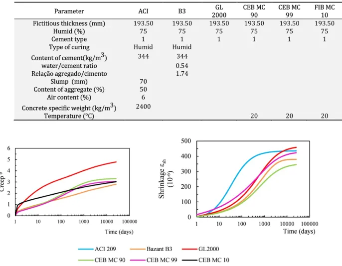
In this section the influence of the ACI, B3, GL, CEB-MC90, CEB-MC99 and FIB-MC 2010 model codes on the η

response and stress distribution is studied. Material properties are listed in Table 2. In Figure 14 are depicted the creep and shrinkage curves for the period of interest. As it can be seen, the final creep coefficient and shrinkage strain vary in the range of 1 to 5 and 350E-06 to 460E-06, respectively (i.e. none procedure was used to obtain the same end values). The stress distributions shown in Figures 15-16 for the fixed end and mid-span, respectively, are almost similar, with exception of the ACI model, which predicted higher initial stresses (around 3 MPa) before loading is applied. This is due to the highest shrinkage strain at which the RC slab is exposed according to this model, e.g. the shrinkage strain at 28 days is 200E-06, whereas the second reported highest strain is 100E-06. Also, the ACI shrinkage curve overcomes the other ones during the period of 7 to 10000 days. Surprisingly, the CEB MC99 and FIB MC results better adjusted Macorini et al.’s ones. The η value increases with time approaching to 1.0 for all models as shown in Figure 17. The η variation along the beam axis is depicted in Figure 18 besides some code results. All models predict similar patterns at 28 days with exception of the ACI model, but in all cases

η approaches to 1.0 at the long-term.

Table 2: Material properties.

Parameter ACI B3 ₂₀₀₀GL CEB MC ₉₀ CEB MC ₉₉ FIB MC ₁₀

Fictitious thickness (mm) 193.50 193.50 193.50 193.50 193.50 193.50

Humid (%) 75 75 75 75 75 75

Cement type 1 1 1 1 1 1

Type of curing Humid Humid

Content of cement(kg/m3) 344 344

water/cement ratio 0.54

Relação agregado/cimento 1.74

Slump (mm) 70

Content of aggregate (%) 50

Air content (%) 6

Concrete specific weight (kg/m3) 2400

(16)

(17)

Figure 16: Stress distribution in the middle fiber of concrete slab at the mid-span (nonlinear viscoelastic analysis with shrinkage and cracking).

(18)

Figure 17: Variation with time of effective width ratio at the mid-span and fixed end (nonlinear viscoelastic with shrinkage and cracking).

5.1.6 Effect of ultimate tensile concrete strain on the effective width ratio

(19)

in the middle fiber of the RC slab using the FIB MC 2010 code. As it may be observed, practically the stress distri-butions at the mid-span remain unchanged at all times.

(20)

sented the η evolution at mid-span and fixed end with time. As it may be observed, the η parameter reaches a minimum value of 0.85 and 0.5 at the fixed end and mid-span, respectively, immediately after loading is applied at 28 days, thereafter η approaches to 1.0 at the long-term. This is valid for almost all εtu values with exception of

εtu= 1.0E-03, in which the η value cannot be calculated after 55 days since concrete stresses are zero at the fixed end. In Eq. 4 is proposed an expression for evaluating the effective width ratio at the short-term along the beam axis for the present example (i.e. 𝑏/𝐿 = 0.12, where 𝑏 = 3 m and 𝐿 = 25 m are the current half slab width and span length, respectively). This expression is plotted in Figure 22 beside the results obtained for all studied creep and shrinkage models. As it may be observed, the present formula agrees with the FE numerical results consider-ing concrete creep, shrinkage and crackconsider-ing. Nevertheless, more parametric studies are needed with other values of span/width ratios, slab thicknesses and shear connection configurations for completeness.































5 .

0

4 .

0 /

4 .

0

15 .

0

36 .

1 /

4 .

2

15 .

0

7 .

0 /

2 /

L

x

L

x

L

x

L

x

L

x

L

x

L

x



(4)

(a) 𝜀 = 1.0E-03. (b) 𝜀 = 2.0E-03.

(c) 𝜀 = 3.0E-03. (d) 𝜀 = 4.0E-03.

(21)

(a) 𝜀 = 1.0E-03. (b) 𝜀 = 2.0E-03.

(c) 𝜀 = 3.0E-03. (d) 𝜀 = 4.0E-03.

Figure 20: Stress distribution in the middle fiber of RC slab at the fixed end for different ultimate tensile strains (FIB MC 2010).

(22)

(a) 𝜀 = 1.0E-03. (b) 𝜀 = 2.0E-03.

(c) 𝜀 = 3.0E-03. (d) 𝜀 = 4.0E-03.

Figure 21: Variation of effective width ratio according to ultimate concrete tensile strain (FIB MC 2010).

(23)

4 CONCLUSIONS

In this work, a finite element based approach is presented for the analysis of non-pre-stressed steel-concrete composite beams under service loads. The model is able to trace the complete nonlinear long-term response of the structure considering concrete creep, shrinkage and cracking of the RC slab. The model is used to carry out a comprehensive study for the effective width evaluation of a composite girder bridge. The obtained FE results ex-pressed in terms of short-term and long-term effective width ratios are compared with other formulations based on some standard codes (ASSTHO, EC4, NBR 8800 and GB 50017) and researches formulas (Yuan et al. 2016, Gara et al. 2009 and Zhu et al. 2017). It is important to mention that the present conclusions should be taken as an initial reference until more experimental data about the effective width variation with time is available. The fol-lowing conclusions can be draw from this study:

• In most responses, the present FE results corroborate Macorini et al’s results at the mid-span and fixed end at all times for all analyses. Differences are encountered for concrete stress distributions mainly at the fixed and for reinforcing bar stresses at the long-term. These differences can be attributed to the manner in which cracking strain are calculated in each constitutive model. Surprisingly, Macorini et al.’s results, which used CEB MC 90, are better adjusted by the current FIB MC 2010 model. It is important to highlight that Macorini et al.’s results constitutes a reference until more experimental data or analytical solutions are available. • The ACI model predicted the highest concrete shrinkage strain since the beginning of the analysis; therefore it yielded a kind of different response in relation to other models.

• The FE results indicate that effective width ratios vary quite irregularly along the beam axis for all analyses (viscoelastic, viscoelastic with shrinkage and viscoelastic with shrinkage and cracking) at the short-term, but it approaches to 1.0 at the long-term for all analyses including shrinkage and/or cracking. Then concrete cracking and shrinkage redistributes concrete stresses

uniformly with time.

• The slab effective width can be evaluated with safety using the middle layer of the RC slab for the present example. This has been corroborated with a more robust through-thickness integration procedure.

•The slab thickness criterion of the Chinese regulation GB50017 imposes a lower limit of 0.5 for the effective width ratio for all analyzed cases.

•For a more realistic analysis including concrete creep, shrinkage and cracking, the effective width ratio predicted by the ASSHTO specification corroborates the long-term effective width ratio predicted by the present numerical model. The GB50017 regulation excluding the thickness criterion also acceptably matches this value although with less accuracy at the fixed end zone. Meanwhile, the effective width ratios calculated with the NBR 8800, EC4 and GB50017 (including the slab thickness criterion) specifications are considerably more conservative along the beam axis.

•None of the aforementioned regulations accompanies the short-term effective width irregular pattern along the beam axis shown in this study. Only Zhu et al.’s method produced a similar trend. Yuan et al.’s method yielded a constant effective width ratio 0.68, which is on the safe side at all times, while Gara et al.’s method provided higher effective width ratios on the unsafe side at the mid-span for the short-term.

•At the serviceability stage, the use of modular ratios is adequate only for the viscoelastic analysis. For other analyses including concrete shrinkage and/or cracking, the modular ratios, which are commonly used in design practice, drastically differ from the predicted stress ratios of rebar to concrete.

•In spite of the short-term effective width ratio variation along the beam axis, it could be necessary to calculate the slab effective width only at the more requested cross sections in flexure. This is because in design practice, the calculated reinforcement at critical sections is extended to the non-critical ones, thus creating an excessive flexural capacity at these locations.

•In practical terms, the effective width ratio at mid-span and fixed end approaches to 1.0 at the long-term, independently of the chosen creep and shrinkage model for an ultimate tensile concrete strain value 0.1. When the FIB MC 2010 model is fixed in the analysis, the use of different ultimate tensile strains does not bring any substantial change on the stress distributions and effective width ratios at mid-span at all times. At the fixed end, its influence is also not relevant for ultimate tensile strains greater or equal than 2.0E-3, only for values around 1.0E-3 (which enforces a very severe cracking process) concrete stresses progressively drops to zero with time; being necessary in this situation to use the effective width ratio of the reinforcing bar stresses. Thus, it could be said in practical terms that ultimate tensile concrete strain does not influence significantly the effective width value for the studied example. Also, there is not significant difference for results calculated with ultimate tensile strains of 4.0E-3 and 0.1.

•It has been reported by Nie et al. (2008) that effective width ratios at collapse loads approach to 1.0 due to stress redistribution. Here, the same conclusion is obtained for the long-term serviceability analysis of a composite girder bridge with 𝑏/𝐿 = 0.12, where 𝑏 = 3 m and 𝐿 = 25 m are the current half slab width and span length, respectively, including concrete creep, shrinkage and cracking.

(24)

AASHTO (2012), AASHTO LRFD bridge design specifications. American Association of State Highway and Trans-portation Officials; Washington, D.C. United States.

Amadio C., Fedrigo, C., Fragiacomo M. and Macorini, L. (2004), Experimental evaluation of effective width in steel-concrete composite beams, Journal of Constructional Steel Research., 60(2), 199-220.

Arockiasamy M. and Sivakumar, M. (2005),Time dependent behavior of continuous composite integral abutment bridges, Practice Periodical on Structural Design and Construction,10(3), 161-170.

Baskar, K., Shanmugam, N.E and Thevendran, V. (2002), Finite element analysis of steel-concrete composite plate girder, J. Struct. Eng., 128(9), 1158-1168.

Bazant, Z. P., Baweja, S., (1995). Creep and shrinkage prediction model for analysis and design of concrete struc-tures-Model B3. Materials and Structures 28:357–365.

Comité Euro-International du Béton (CEB 1993), CEB-FIP Model Code 1990, CEB Bulletin d’Information No 213/214, Committee European du Béton-Fédération Internationale de la Précontrainte; Lausanne, Switzerland.

Comité Euro-International du Béton (CEB 1999), Structural concrete-Textbook on behavior, design and Perfor-mance, Updated Knowledge of the CEB-FIP Model code 1990, fib bulletin 2, V. 2, Federation Internationale du Beton; Lausanne, Switzerland.

Castro, J. M., Elghazouli, A. Y. and Izzuddin, B. A. (2007), Assessment of effective slab widths in composite beams, Journal of Constructional Steel Research, 63(10), 1317-1327.

Chen, S. and Zhang Z. (2006), Effective width of a concrete slab in steel-concrete composite beams prestressed with external tendons, Journal of Constructional Steel Research, 62(5), 493-500.

Chiewanichakorn, M., Aref, A.J., Chen S.S. and Ahnll-S.(2004), Effective flange width definition for steel-concrete composite bridge girder, J. Struct. Eng., 130(12), 2016-2031.

Dias, M.M., Tamayo, J.L.P., Morsch, I.B. and Awruch, A.M. (2015), Time dependent finite element analysis of steel-concrete composite beams considering partial interaction, Comput. Concrete, 15(4), 687-707.

Dezi, L., Gara, F., Leoni, G. and Tarantino, A.M. (2001), Time-depedent analysis of shear-lag effect in composite beam, Journal of Engineering Mechanics, 127(1), 71-79.

Dezi, L., Gara, F. and Leoni, G.(2006), Effective slab width in prestressed twin-girder composite decks, J. Struct. Eng., 132(9), 1358-1370.

EC4 (2005), Design of composite steel and concrete structures – Part 2: General rules and rules for bridges. Euro-pean Committee for Standardization (Eurocode 4); Brussels, Belgium.

Fédération Internationale du Béton (FIB 2010), fib Bulletin 70: Code-type models for structural behaviour of con-crete: Background of the constitutive relations and material models in the fib Model Code for Concrete Structures, Model Code for Concrete Structures, Fédération Internationale du Béton; Lausanne, Switzerland.

Gadner, N. J. and Lockman, M. J., (2001). Design provisions for drying shrinkage and creep of normal strength concrete. ACI Materials Journal 98:159–167.

(25)

Galuppi, L. and Carfagni, G.R. (2016), Effective width of the slab in composite beams with nonlinear shear connec-tion, Journal of Engineering Mechanics, 142(4), 04016001-1-10.

GB50017 (2003). Code for design of steel structures. National Standard of the People’s Republic of China. Beijing, China.

Liang, Q. Q., Uy, B., Bradford, M.A. and Ronagh, H.R. (2005), Strength analysis of steel-concrete composite beams in combined bending and shear, Journal of Structural Engineering, 131(10), 1593-1600.

NBR8800 (2008). Design of steel and composite structures of buildings.Brazilian Association of Technical Regula-tions. Rio de Janeiro, RJ. Brazil.

Nie, J., Tian, C., and Cai, C. (2008), Effective width of steel-concrete composite beams at ultimate strength state, Engineering Structures, 30(5), 1396-1407.

Nie, J., and Tao, M. (2012), Slab spatial composite effect in composite frame system.I: Effective width for ultimate load capacity, Engineering Structures, 38(January), 171-184.

Macorini, L., Fragiacomo, M., Amadio, C. and Izzuddin, B.A. (2006), Long-term analysis of steel-concrete composite beams: FE modelling for effective width evaluation, Engineering Structures, 28(8), 1110-1121.

Rex, O.C. and Easterling, W.S. (2000), Behavior and modeling of reinforced composite slab in tension, Journal of Structural Engineering, 126(7), 764-771.

Salama, T. and Nassif, H.H. (2011), Effective flange width for composite steel beams, The Journal of Engineering Research, 8(1), 28-43.

Tamayo, J.L.P. and Awruch, A.M. (2016), Numerical simulation of reinforced concrete nuclear containment under extreme loads,Struct. Eng. Mech., 58(5), 799-823.

Tamayo, J.L.P., Morsch, I.B. and Awruch, A.M. (2015), Short-time numerical analysis of steel-concrete composite beams, J Braz. Soc. Mech. Sci. Eng., 37(4), 1097-1109.

Tamayo, J.L.P., Morsch, I.B. and Awruch, A.M. (2013), Static and dynamic analysis of reinforced concrete shells, Lat. Am. j. solid.struct.,10(6), 1109-1134.

Moscoso, A.M., Tamayo, J.L.P. and Morsch, I.B. (2017), Numerical simulation of external pre-stressed steel-concrete composite beams,Comput. Concrete, 19(2), 191-201.

Wang, Y. H. and Nie, J. G. (2015), Effective flange width of steel-concrete composite beam with partial openings in concrete slab, Materials and Structures, 48(10), 3331-3342.

Xue, W., Ding, M., He, C., and Li, J. (2008), Long-term behavior of prestressed composite beams at service loads for one year, J. Struct.Eng, 134(6), 930-937.