www.hydrol-earth-syst-sci.net/20/2611/2016/ doi:10.5194/hess-20-2611-2016
© Author(s) 2016. CC Attribution 3.0 License.
Machine learning methods for empirical streamflow simulation:
a comparison of model accuracy, interpretability, and
uncertainty in seasonal watersheds
Julie E. Shortridge1, Seth D. Guikema2, and Benjamin F. Zaitchik3
1Department of Geography and Environmental Engineering, Johns Hopkins University, Baltimore, MD, USA 2Department of Industrial and Operations Engineering, University of Michigan, Ann Arbor, MI, USA 3Department of Earth and Planetary Sciences, Johns Hopkins University, Baltimore, MD, USA
Correspondence to:Julie E. Shortridge ([email protected])
Received: 25 September 2015 – Published in Hydrol. Earth Syst. Sci. Discuss.: 28 October 2015 Revised: 15 April 2016 – Accepted: 29 May 2016 – Published: 4 July 2016
Abstract.In the past decade, machine learning methods for empirical rainfall–runoff modeling have seen extensive de-velopment and been proposed as a useful complement to physical hydrologic models, particularly in basins where data to support process-based models are limited. However, the majority of research has focused on a small number of methods, such as artificial neural networks, despite the de-velopment of multiple other approaches for non-parametric regression in recent years. Furthermore, this work has of-ten evaluated model performance based on predictive accu-racy alone, while not considering broader objectives, such as model interpretability and uncertainty, that are important if such methods are to be used for planning and manage-ment decisions. In this paper, we use multiple regression and machine learning approaches (including generalized ad-ditive models, multivariate adaptive regression splines, arti-ficial neural networks, random forests, and M5 cubist mod-els) to simulate monthly streamflow in five highly seasonal rivers in the highlands of Ethiopia and compare their per-formance in terms of predictive accuracy, error structure and bias, model interpretability, and uncertainty when faced with extreme climate conditions. While the relative predictive per-formance of models differed across basins, data-driven ap-proaches were able to achieve reduced errors when com-pared to physical models developed for the region. Meth-ods such as random forests and generalized additive models may have advantages in terms of visualization and interpre-tation of model structure, which can be useful in providing insights into physical watershed function. However, the
un-certainty associated with model predictions under extreme climate conditions should be carefully evaluated, since cer-tain models (especially generalized additive models and mul-tivariate adaptive regression splines) become highly variable when faced with high temperatures.
1 Introduction
Hydrologists and water managers have made use of ob-served relationships between rainfall and runoff to predict streamflow ever since the creation of the rational method in the 19th century (Beven, 2011). However, the development of increasingly sophisticated machine learning techniques, combined with rapid increases in computational ability, has prompted extensive research into advanced methods for data-driven streamflow prediction in the past decade. Artificial neural networks (ANNs), regression trees, and support vector machines have been shown to be powerful tools for predic-tive modeling and exploratory data analysis, particularly in systems that exhibit complex, non-linear behavior (Soloma-tine and Ostfield, 2008; Abrahard and See, 2007).
ef-forts to merge satellite data with in situ observations to mon-itor climate and hydrology has made acceptable climate and streamflow data more widely available in data-poor regions. Because obtaining measurement-based estimates of soil hy-draulic parameters or details on hydrologically relevant land management activities can be more difficult, empirical mod-els may be particularly useful in these locations.While many criticize these approaches as “black boxes” with no rela-tionship to underlying physical processes (See et al., 2007), a number of studies have demonstrated how empirical ap-proaches can be used to gain insights about physical sys-tem function (e.g., Han et al., 2007; Galelli and Castelletti, 2013a). Additionally, improvements in interpretation and vi-sualization methods can make complex models more easily interpretable (Sudheer and Jain, 2004; Jain et al., 2004). Fi-nally, data-driven models can be useful in identifying sit-uations where observed data disagree with what would be predicted based on conceptual models, and thus identify as-sumptions regarding runoff generation processes that may be incorrect (Beven, 2011).
While there have been some applications of alternative machine learning methods, such as support vector machines (Asefa et al., 2006; Lin et al., 2006) and regression-tree-based approaches (Iorgulescu and Beven, 2004; Galelli and Castelletti, 2013a) for streamflow simulation, the vast ma-jority of research has focused on artificial neural networks (Solomatine and Ostfield, 2008). While they have demon-strated impressive predictive accuracy in a number of dif-ferent contexts, excessive parameterization of ANNs can re-sult in overfit models that are not generalizable to unseen data (Iorgulescu and Beven, 2004; Gaume and Gosset, 2003). While methods exist to avoid overfitting, such as cross vali-dation and bootstrapping, these methods are not always em-ployed (Solomatine and Ostfield, 2008). A review by Maier et al. (2010) found that relatively few studies evaluated model performance based on parameters such as Akaike informa-tion criterion that would lead to parsimonious models that are likely to be more generalizable and interpretable. This can lead to complex models that only result in modest im-provements (or no imim-provements at all) over much simpler approaches (Gaume and Gosset, 2003; Han et al., 2007).
Even outside of a hydrology context, it has been argued that ANNs are better suited for problems aimed at predic-tion without any need for model interpretapredic-tion, rather than those where understanding the process generating predic-tions and the role of input variables is important (Hastie et al., 2009). Given the importance that this interpretation plays in understanding the contexts in which a hydrologic model is appropriate and reliable, the strong opinions surrounding the use of ANNs for water resources management are per-haps not surprising. To address this issue, a number of studies have focused on highlighting the structure and mechanism by which machine learning models make predictions to confirm their physical realism and gain insight into physical water-shed function. For example, some studies have demonstrated
how internal ANN structure corresponds to physical hydro-logic processes (Wilby et al., 2003; Jain et al., 2004; Sudheer and Jain, 2004), while others have shown how variable se-lection and importance can be used to gain insights about model structure and runoff generating processes (Galelli and Castelletti, 2013a, b). While these studies demonstrate that a number of methods exist for characterizing model structure, they generally focus on a single model type and thus provide little insight into the comparative ease with which different model types can be interpreted.
While a number of comparison studies exist that apply multiple empirical models to a given problem, finding gen-eralizable insights from these studies is hindered because of the limited number of models and data sets evaluated. Per-haps the most comprehensive comparison to date is that of Elshorbagy et al. (2010a, b), who compared six methods for data-driven modeling of daily discharge in the Ourthe river in Belgium. This work found that linear models were able to perform comparably to much more complex meth-ods when the data content of the models was limited, or when system input–output behavior was close to linear. How-ever, other studies have demonstrated the value of using more complex approaches when modeling more complex rainfall– runoff behavior (e.g., Abrahart and See, 2007; Asefa et al., 2006). The differing results obtained across these studies in-dicate that no single method is likely to be suitable for all basins, timescales, or applications.
However, it is important to recognize that predictive ac-curacy alone is not necessarily sufficient justification for ap-plying a model to a given problem. Models should not only be accurate but also be fit for purpose (Beven, 2011; Van Griensven et al., 2012). For instance, accurate representation of low return period flows is more important in a flood fore-casting model than one aimed at predicting average amounts of water available for withdrawal and human consumption. Similarly, the ability to provide insights into physical water-shed function may be more important in basins where land-use change could alter the hydrologic regime, compared to a basin that is heavily urbanized and expected to remain so. The use of multiple objective functions in training data-driven models can address this to some degree by identify-ing models that provide sufficient balance between different performance objectives, such as accurate representation of different portions of the flow hydrograph (De Vos and Rient-jes, 2008). However, more refined model training procedures will not necessarily address other aspects of model perfor-mance that make it suitable for planning purposes, such as interpretability (Solomatine and Ostfield, 2008). More com-prehensive consideration of model strengths and limitations should be standard practice in model development and selec-tion, rather than simply evaluating global error metrics.
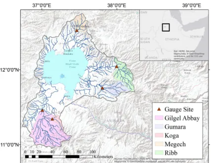
Figure 1.Map of Lake Tana and surrounding rivers.
Tana basin in Ethiopia. This study region was selected as it provides insights into the use of data-driven models for streamflow simulation in tropical regions of the world that are underrepresented in existing studies. For instance, a re-view of 210 articles on water resource applications of ANNs found that over three-quarters of the studies evaluated were conducted in North America, Europe, Australia, or temperate east Asia (Maier et al., 2010). Existing studies conducted in tropical regions generally apply a single methodology to the basin of interest and evaluate predictive accuracy alone (see, for instance, Machado et al., 2011; Chibanga et al., 2003; An-tar et al., 2006; Aqil et al., 2007), making it difficult to find generalizable insights into the relative advantages of different modeling approaches in these regions. Better development of data-driven models for these regions has the potential to be particularly valuable because data limitations and complex hydrodynamic processes often hinder the use of physical wa-tershed models, but relatively long time series of streamflow, precipitation, and temperature may be available at a monthly timescale. These data, combined with information on rele-vant landscape change (in particular, the expansion of agri-cultural land cover), can be leveraged to create reasonably accurate empirical models.
Models are compared not only in terms of their predic-tive accuracy but also in terms of model error structure and the implications that this structure may have for water re-source applications. Additionally, we evaluate the methods by which model structure and predictor variable influence can be evaluated to gain insights into physical system func-tion for each model type. Finally, we assess the suitability of using different model types for climate change impact assess-ment by comparing model uncertainty in projections made
for increasingly extreme climate conditions. The overall ob-jective of this research is not to identify a single best model, but rather to highlight some of the strengths and limitations of different approaches, as well as demonstrate important is-sues that should be kept in mind for model comparisons in the future.
2 Data and methods 2.1 Study area
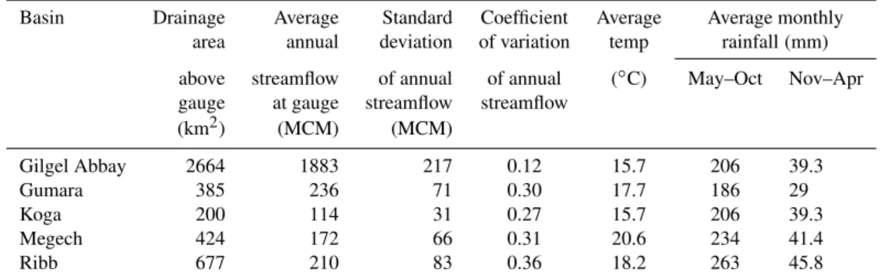
Table 1.Study basin characteristics over the evaluation period of 1961–2004.
Basin Drainage Average Standard Coefficient Average Average monthly
area annual deviation of variation temp rainfall(mm)
above streamflow of annual of annual (◦C) May–Oct Nov–Apr
gauge at gauge streamflow streamflow
(km2) (MCM) (MCM)
Gilgel Abbay 2664 1883 217 0.12 15.7 206 39.3
Gumara 385 236 71 0.30 17.7 186 29
Koga 200 114 31 0.27 15.7 206 39.3
Megech 424 172 66 0.31 20.6 234 41.4
Ribb 677 210 83 0.36 18.2 263 45.8
Approximately 2.6 million people live in the basin, and are largely settled in rural areas and reliant on rainfed subsis-tence agriculture. This makes the region quite vulnerable to climate variability and change, and a number of water re-sources infrastructure projects are planned to better manage this vulnerability and support economic development (Ale-mayehu et al., 2010). This includes the recent construction of the Tana–Beles hydropower transfer tunnel and the Koga River irrigation reservoir, as well as five other reservoirs planned for construction in the next 10–20 years (Alemayehu et al., 2010). To better understand the potential implications of this development, extensive effort has been put towards developing rainfall–runoff models for the Lake Tana basin, as well as other areas of the Ethiopian highlands with similar characteristics (Van Griensven et al., 2012). Many of these studies rely on Soil and Water Assessment Tool (SWAT) models, although there are some that use water balance ap-proaches (Van Griensven et al., 2012). While these mod-els have in some cases demonstrated reasonably high accu-racy, previous evaluations were largely based on the Nash– Sutcliffe efficiency (NSE; Nash and Sutcliffe, 1970) which can be a flawed performance metric in highly seasonal wa-tersheds (Schaefli and Gupta, 2007; Legates and McCabe Jr., 1999). More importantly, the limited data available for phys-ical parameterization of these models required a heavy re-liance on model calibration, which sometimes resulted in parameterization schemes that are inconsistent with physi-cal understanding of the region’s hydrology (Steenhuis et al., 2009; Van Griensven et al., 2012). Furthermore, a number of studies relied on empirical relationships, such as curve num-bers and the Hargreaves equation, that were developed for temperate regions (e.g., Mekonnen et al., 2009; Setegn et al., 2009). While these limitations are likely to introduce con-siderable uncertainty into model projections, particularly in situations where climatic or environmental conditions differ from those experienced in the calibration period, few studies from this region of Ethiopia include any sort of uncertainty analysis in model predictions. Empirical models could pro-vide a useful complement to physical models developed for the region by providing insights into physical system
func-tion and allowing for more comprehensive uncertainty anal-ysis.
2.2 Data and model development
out-of-sample predictive accuracy of the models, further suggesting that it was a valuable addition.
Two general formulations for the empirical models were evaluated. The first (referred to below as the standard model formulation) was
log Qb,t
=f Pb,t, Pb,t−1, Pb,t−2, Tb,t, Tb,t−1, Tb,t−2,
AgLCb,t
+εb,t, (1)
where Qb,t is the monthly streamflow in river b at time period t; Pb,t and Tb,t are the monthly total precipitation and average temperature in river basin b at time period t; AgLCb,t is the total percentage of agricultural land cover in basinbat timet; andεb,t is the model error. The subscripts
t−1 andt−2 indicate lagged measurements from 1 and 2 months prior, and were included to roughly account for stor-age times longer than 1 month that could impact streamflow in each river. While the exact time of concentration is not known in each basin, the minor influence of climate condi-tions at 2 months prior suggests that climate condicondi-tions from beyond this time period do not contribute significantly to flow variability. The function f represents a general func-tion that differed between the specific models assessed and is discussed in more detail below. The logarithm of monthly streamflow was used as a response variable to keep model predictions positive. The distribution of streamflow data and log-transformed streamflow values in each basin is shown in Fig. S1 in the Supplement.
In the second formulation, streamflow and climate anoma-lies were used as the response and predictor variables to bet-ter account for the highly seasonal nature of streamflow and precipitation in the region. Streamflow anomalies were cal-culated for each observation by subtracting the long-term av-erage streamflow for that month (m) from the observed value and dividing this number by the long-term standard devia-tion of that month’s streamflow as in Eq. (2). Anomaly val-ues thus represent how streamflow in a given month com-pares to the long-term average flow for that month; for stance, an anomaly value of 1.0 for June of 1990 would in-dicate that streamflow in that month was 1 standard devia-tion higher than the average June flow from 1961 to 2004. This procedure was repeated for precipitation and tempera-ture, and these values were then used to fit models of the form described in Eq. (3). In each month of the time series, the model estimates the flow relative to the long-term aver-age flow for that month, based on whether temperature and precipitation values were greater or less than their long-term averages, as well as the percentage of agricultural land cover in that month of the time series. In this sense, the anomaly values are calculated based on climatic and land cover condi-tions that vary through time. These anomaly values are then converted back to raw flow values based on the long-term average and standard deviation of flow for that month. The distribution of streamflow anomaly values in each basin are shown in Fig. S1.
QANb,t = Qb,t−Qb,m
sd (Q−b, m) (2)
QANb,t =fPb,tAN, Pb,tAN−1, Pb,tAN−2, Tb,tAN, Tb,tAN−1, Tb,tAN−2,
AgLCb,t
+εb,t (3)
Six different types of models were compared using each for-mulation in each basin:
1. A Gaussian linear regression model (GLM) using the basic stats package in the R statistical computing soft-ware (R Development Core Team, 2014)
2. Gaussian generalized additive model (GAMs) are semi-parametric regression approaches where the response variable is estimated as the sum of smoothing functions applied over predictor variables. These functions allow the model to capture non-linear relationships between the predictor and response variables without a priori as-sumptions about the form (e.g., quadratic, logarithmic) of these functions, and are fit using penalized likelihood maximization to prevent model overfitting (Hastie and Tibshirani, 1990). GAMs were fit using the mgcv pack-age in R (Wood, 2011).
3. Multivariate adaptive regression splines (MARS) are a non-parametric regression approach where the response variable is estimated as the sum of basis functions fit to recursively partitioned segments of the data (Friedman, 1991). MARS models were fit using the earth package in R (Milborrow, 2015).
4. ANNs are a non-parametric regression approach repre-sented by a network of nodes and links that connects predictor variables to the response variable. Each link in the network represents a function that maps the input nodes into the output node (Ripley, 1996). ANN mod-els were fit using the nnet package in R (Venables and Ripley, 2013).
5. Random forest (RFs) are a rule-based, non-parametric regression approach where the model prediction is cre-ated by averaging the predicted value from multiple regression trees which are trained on separate boot-strapped resamples of the data. Each tree is fit using a small, randomly selected subset of predictor variables, resulting in reduced correlation between trees (Breiman, 2001). Random forest models were fit using the ran-domForest package in R (Liaw and Wiener, 2002). 6. M5 models are a rule-based, non-parametric regression
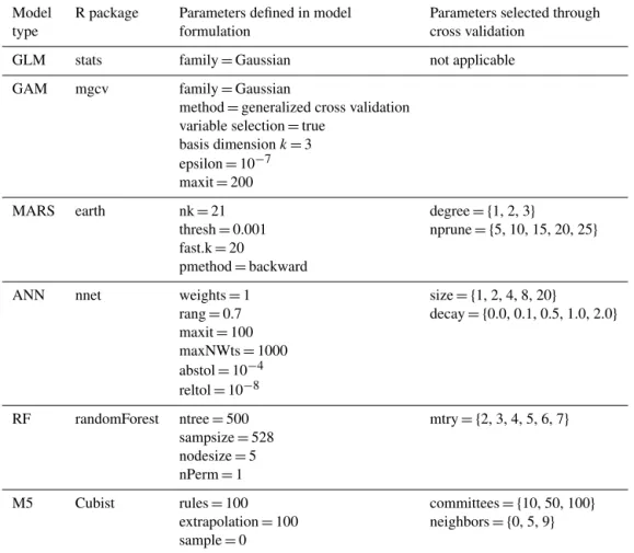
Table 2.Model parameters evaluated through cross validation.
Model R package Parameters defined in model Parameters selected through
type formulation cross validation
GLM stats family=Gaussian not applicable
GAM mgcv family=Gaussian
method=generalized cross validation variable selection=true
basis dimensionk=3 epsilon=10−7 maxit=200
MARS earth nk=21 degree= {1, 2, 3}
thresh=0.001 nprune= {5, 10, 15, 20, 25}
fast.k=20
pmethod=backward
ANN nnet weights=1 size= {1, 2, 4, 8, 20}
rang=0.7 decay= {0.0, 0.1, 0.5, 1.0, 2.0}
maxit=100 maxNWts=1000 abstol=10−4 reltol=10−8
RF randomForest ntree=500 mtry= {2, 3, 4, 5, 6, 7}
sampsize=528 nodesize=5 nPerm=1
M5 Cubist rules=100 committees= {10, 50, 100}
extrapolation=100 neighbors= {0, 5, 9}
sample=0
7. A climatology model that simply predicted each month’s streamflow as equivalent to the long-term av-erage streamflow for that month was included for com-parison purposes.
2.3 Model evaluation
When using non-parametric regression approaches, it is im-portant to avoid overfitting a model to a given data set be-cause this can result in large errors in out-of-sample predic-tions (Hastie et al., 2009). To avoid model overfit, the caret package in R (Kuhn, 2015) was used to determine model pa-rameters for the MARS, ANN, RF, and M5 models. This package uses resampling to evaluate the effect that model parameters have on the model’s predictive performance and chooses the set of parameters that minimizes out-of-sample error (Kuhn, 2015). In this evaluation, 25 bootstrap resam-ples of the training data set were generated for each parame-ter value to be assessed. A model was fit using each bootstrap sample and used to predict the remaining observations and the parameter values that minimized average RMSE across all resamples. Details on the specific parameters evaluated for each model are presented in Table 2. While the develop-ment of more complex structures is possible for some
mod-els, this process can result in overparameterization and poor model performance (Gaume and Gosset, 2003; Han et al., 2007). Additionally, the use of a standardized parameteriza-tion procedure allows for a more even comparison between different model types.
from the use of a single calibration and validation data set (Elshorbagy et al., 2010a; Han et al., 2007).
MAE was included as an error metric because it pro-vides a simple and easily interpretable measure of error on the same scale as observed flow volumes. While NSE val-ues are acknowledged to be a flawed performance metric in highly seasonal watersheds where seasonal fluctuations con-tribute to a substantial portion of flow variability (Schaefli and Gupta, 2007; Legates and McCabe Jr., 1999), this met-ric was included to provide a rough comparison of how em-pirical model performance compared to the performance of physical models developed for the region. The use of alter-native error metrics has been discussed extensively in the lit-erature (for instance, Pushpalatha et al., 2012; Mathevet et al., 2006; Criss and Winston, 2008), and could provide addi-tional insights into what contributes to predictive capabilities of different model formulations. However, this work exam-ined predictive accuracy based on MAE and NSE alone to allow for greater focus on how models differ in terms of er-ror structure and uncertainty.
As a rough point of comparison for the statistical mod-els developed in this research, we also evaluated discharge estimates derived from a process-based hydrological model. The model used in this application is the Noah Land Sur-face Model version 3.2 (Noah LSM; Ek et al., 2003; Chen et al., 1996). Noah LSM was implemented for offline sim-ulations of the Lake Tana basin at a gridded spatial resolu-tion of 5 km for the period 1979–2010 using a time step of 30 min. Meteorological forcing was drawn from the Prince-ton 50-year reanalysis data set (Sheffield et al., 2006), down-scaled to account for Ethiopia’s steep terrain using MicroMet elevation correction equations (Liston and Elder, 2006). The Princeton reanalysis was selected because it provides rel-atively high-resolution meteorological fields, including all variables required to run a water and energy balance LSM like Noah, for the period 1948–present. While higher res-olution and possibly higher quality data sets are available for recent years, this longer data set was utilized to compare the process-based model to statistical models developed for a long historical period. Soil parameters for the Noah simu-lation were drawn from the FAO global soil database, land use was defined according to the United States Geological Survey (USGS) global 1 km land cover product, and vege-tation fraction was derived from MODerate Imaging Spec-troradiometer (MODIS) imagery. Land cover was treated as a static parameter over the full length of the simulation, as spatially complete estimates of historical land use were not available at the required resolution and specificity.
The highest performing model in each basin based on MAE was retained for more detailed evaluation of model error structure, covariate influence, and uncertainty in cli-mate change sensitivity analysis. To generate a complete time series of out-of-sample model predictions for error analy-sis, the holdout cross-validation procedure was repeated for the highest performing standard-formulation and
anomaly-formulation models for each basin, but this time holding out a single year of observations in each iteration. The predic-tions from this cross validation were used to evaluate how model error structure might impact model predictions used for water resource applications. The influence of different predictor variables on model predictions was also assessed for the highest performing model in each basin after being fit to the complete data set. Each predictor variable was as-sessed using metrics for covariate importance and influence that are unique to that model type, demonstrating how mod-els could be used to gain physical insights about data-scarce regions, and the mechanisms for generating these insights for each type of model. Partial dependence plots (Hastie et al., 2009) were also generated for each covariate for the high-est performing model in each basin to provide insights about how covariate influence compared across different basins and model types.
Finally, two evaluations were conducted to assess uncer-tainty in model projections of streamflow under increasingly extreme climate conditions to better understand the impli-cations of using different model formulations for climate change impact studies. Model projections of streamflow in different climate conditions are likely to be accompanied by considerable uncertainty, particularly when climate condi-tions exceed those experienced historically. To assess this un-certainty, the best performing model in each basin was used to generate streamflow predictions for (1) changes in tem-perature from 0 to 5◦C, (2) changes in precipitation from −30 to+30 %, (3) an increase in temperature to 5◦C com-bined with a decrease in precipitation to−30 %, and (4) an increase in temperature to 5◦C combined with an increase
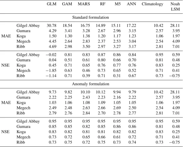
Table 3.Cross-validation errors for each assessed model.
GLM GAM MARS RF M5 ANN Climatology Noah
LSM
Standard formulation
MAE
Gilgel Abbay 30.78 18.54 16.75 14.89 15.11 17.22 10.42 28.11
Gumara 4.29 3.41 3.28 2.67 2.96 3.15 2.57 3.95
Koga 1.50 1.30 1.38 1.20 1.17 1.23 1.06 1.97
Megech 4.45 2.64 2.83 2.37 2.53 3.04 2.54 4.09
Ribb 4.69 2.98 3.50 2.97 3.27 3.17 2.81 7.01
NSE
Gilgel Abbay −0.02 0.81 0.83 0.87 0.86 0.84 0.95 0.59
Gumara 0.04 0.51 0.61 0.80 0.66 0.70 0.81 0.48
Koga 0.45 0.71 0.65 0.76 0.77 0.76 0.83 0.25
Megech −1.85 0.63 0.46 0.73 0.65 0.52 0.71 0.41
Ribb −1.14 0.71 0.39 0.71 0.31 0.67 0.73 −0.75
Anomaly formulation
MAE
Gilgel Abbay 9.73 9.82 10.10 10.12 9.94 9.79 10.42 28.11
Gumara 2.22 2.25 2.43 2.23 2.16 2.22 2.57 3.95
Koga 1.03 1.06 1.08 1.09 1.05 1.05 1.06 1.97
Megech 2.49 2.48 2.63 2.66 2.69 2.50 2.54 4.09
Ribb 2.79 2.76 2.84 2.70 2.78 2.77 2.81 7.01
NSE
Gilgel Abbay 0.95 0.95 0.95 0.95 0.95 0.95 0.95 0.59
Gumara 0.85 0.85 0.82 0.85 0.86 0.86 0.81 0.48
Koga 0.83 0.82 0.81 0.81 0.82 0.82 0.83 0.25
Megech 0.73 0.72 0.65 0.66 0.61 0.72 0.71 0.41
Ribb 0.73 0.75 0.72 0.75 0.73 0.74 0.73 −0.75
3 Results
3.1 Model accuracy and error structure
Table 3 shows the out-of-sample cross-validation errors for each model assessed in each basin. The random forest model had the lowest mean absolute error for the standard-formulation model in four of the five basins, with the M5 model performing best for the Koga basin. These mod-els outperformed the Noah LSM simulations in all basins assessed. The Noah LSM errors are for a single period of analysis and thus do not present an exact corollary to the cross validation performed for the empirical models. Nev-ertheless, the significant increases in errors associated with the Noah LSM model demonstrates the difficulty associated with the use of process-based models in the region, particu-larly when relying on global data sets that may be unreliable at the spatial and temporal resolutions required for physical modeling. Physical models developed for monthly stream-flow prediction in other basins within the Ethiopian high-lands have reported NSE values ranging from 0.53 to 0.92 (Van Griensven et al., 2012), compared to values ranging from 0.71 to 0.87 for the random forest models developed here. If this measure alone was used for model evaluation, these empirical models would generally be classified as hav-ing good performance based on the guidelines suggested by
Moraisi et al. (2007). However, the climatology model out-performs the best standard-formulation models in all basins except Megech, indicating that in the majority of basins the errors from the fitted empirical models are higher than those that result from simply using the long-term monthly average for each month’s prediction. This is due to the fact that sea-sonality accounts for such a large portion of the variability in monthly flow values, and demonstrates how high NSE values can be quite easy to obtain in seasonal basins.
Evaluation of anomaly model errors indicates that the models using this formulation achieve better predictive accu-racy than those using the standard formulation, and are able to outperform the climatology model based on both NSE and MAE in all basins. However, the highest performing mod-els in each basin vary more when the anomaly formulation is used, with the GLM, GAM, random forest, and M5 mod-els all minimizing MAE in different basins. In all basins ex-cept Koga, the highest performing model significantly out-performed the climatology model based on paired Wilcoxon rank-sum tests (Bonferroni-correctedpvalue<0.01).
Figure 2.Autocorrelation in model residuals for the Gilgel Abbay and Ribb rivers.
Figure 3. Example observed and predicted flows from the standard-formulation RF model and anomaly-formulation M5 model for the Gumara River from 1985 to 1991.
and demonstrate that a positive autocorrelation exists at the 12-month time lag. For brevity, only plots for two rivers are shown, although this autocorrelation existed in the standard-formulation models for all basins except Megech (Table 4). This autocorrelation occurs because the standard-formulation models consistently underestimate wet-season streamflow while overestimating dry-season flows, as is ap-parent in hydrographs of observed and predicted streamflow (Fig. 3). Because wet-season flows contribute such a large portion of the total annual flow volume, this results in reg-ular underestimation of aggregate values such as mean an-nual flow (Table 4). This autocorrelation is reduced in the anomaly-formulation models, meaning that they are better able to capture the peak flow volumes experienced in the wet season and do not underestimate mean annual flow to the same degree that the standard-formulation models do.
3.2 Model structure and covariate influence
Evaluating the relationship between predictor covariates and streamflow response can lend insight into the physical pro-cesses underlying runoff generation in each basin. There are two components of this relationship that can be evaluated: how much each covariate contributes to model accuracy
(co-variate importance), and the direction and nature of the re-lationship between covariate values and model response (co-variate influence). In many machine learning models, com-plete description of the all of the mathematical relationships within the model (for instance, through description of each tree comprising a random forest model) is infeasible, requir-ing the use of other mechanisms for understandrequir-ing covari-ate importance and influence. However, because each model type is structured in a different way, these mechanisms differ. This section first describes the mechanisms available for ob-taining insights about covariate influence in each of the high-est performing models. To provide a mechanism for compar-ing results across different basins, each basin model is then assessed using the general approach of partial dependence plots.
intu-Table 4.Residual autocorrelation factors at a 12-month lag for the highest performing standard-formulation and anomaly-formulation models in each basin (with model type in parentheses), and resulting mean annual observed and predicted flow.
Autocorrelation factors Mean annual flow (MCM)
Standard Anomaly Observed Standard Anomaly
Gilgel 0.33 (RF) 0.11 (GLM) 22 925 20 703 22 958
Gumara 0.29 (RF) 0.07 (M5) 2870 2392 2734
Koga 0.04 (M5) 0.10 (GLM) 1383 1333 1386
Megech 0.05 (RF) 0.04 (GAM) 2035 1637 2028
Ribb 0.21 (RF) −0.01 (RF) 2575 1969 2615
itive. For instance, in the Gilgel Abbay model an increase of 1 standard deviation in precipitation results in an increase of 0.22 SDs (standard deviations) in flow. The associated
p value for each coefficient evaluates a null hypothesis that the true coefficient value is equal to 0 given the other covari-ates in the model, and thus has no influence on the response variable.
Evaluating model structure based on regression coeffi-cients is appealing due to their simplicity and familiarity. However, it is important to keep in mind that the above intpretations rely on specific assumptions regarding model er-ror distributions. Examination of fitted model residuals from both basins indicates that errors are autocorrelated in the Koga basin and not normally distributed due to the presence of outliers in both basins. Non-normality and autocorrelation both impact thet andf statistics used to test for the signif-icance of model coefficients, and thus thepvalues for these models are likely biased (Montgomery et al., 2012).
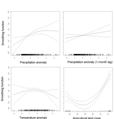
Interpretation of variable influence in GAMs is based on the estimated degrees of freedom (EDF) a covariate’s smoothing function s(Xi)uses within a model (Hastie and Tibushini, 1986). An EDF value of 1 or below indicates a lin-ear function relating the response variable to that covariate, while values greater than 1 represent a non-linear smooth-ing function. An EDF value of 0 indicates that the covariate smoothing function is penalized to 0 (meaning it has no in-fluence on model predictions). In the model for the Megech River, the terms for lagged temperature at 1 and 2 months, as well as precipitation lagged at 2 months were all smoothed to 0. Of the remaining covariates, lagged precipitation has a linear impact on model response, while precipitation, tem-perature, and land cover have non-linear impacts. Smoothing functions can be plotted to gain more insight about these re-lationships (Fig. 4). The functions for precipitation anomaly, lagged (1 month) precipitation anomaly, and agricultural land cover show a positive relationships with streamflow, while the function for temperature anomaly predicts low stream-flow at both high and low anomalies.
P values test the null hypothesis that a covariate’s smooth-ing function is equal to 0, but rest on the assumption that model residuals are homoscedastic and independent (Wood, 2012). Similar to the linear models, residuals in the Megech
Figure 4.Plots of the smoothing functions used in the Megech River GAM. Hash marks along thexaxis indicate observation val-ues of each covariate.
GAM model appear to be both autocorrelated and het-eroscedastic, meaning that a formal statistical interpreta-tion of this value may be inappropriate and that confidence bounds around smoothing functions might be misleading.
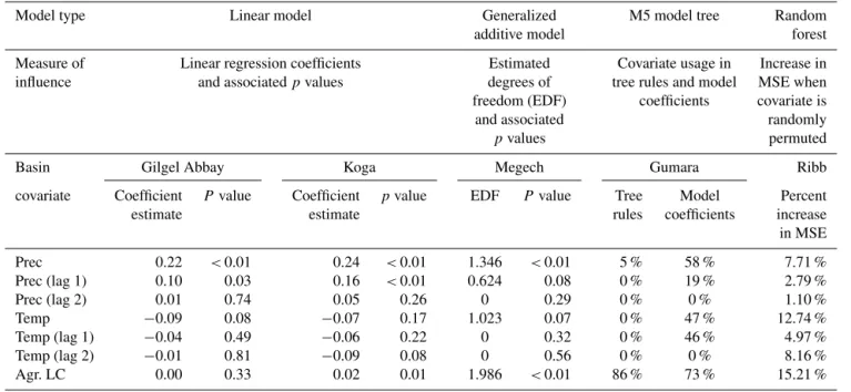
Table 5.Covariate importance measurements from each basin’s model.
Model type Linear model Generalized M5 model tree Random
additive model forest
Measure of Linear regression coefficients Estimated Covariate usage in Increase in
influence and associatedpvalues degrees of tree rules and model MSE when
freedom (EDF) coefficients covariate is
and associated randomly
pvalues permuted
Basin Gilgel Abbay Koga Megech Gumara Ribb
covariate Coefficient P value Coefficient pvalue EDF P value Tree Model Percent
estimate estimate rules coefficients increase
in MSE
Prec 0.22 <0.01 0.24 <0.01 1.346 <0.01 5 % 58 % 7.71 %
Prec (lag 1) 0.10 0.03 0.16 <0.01 0.624 0.08 0 % 19 % 2.79 %
Prec (lag 2) 0.01 0.74 0.05 0.26 0 0.29 0 % 0 % 1.10 %
Temp −0.09 0.08 −0.07 0.17 1.023 0.07 0 % 47 % 12.74 %
Temp (lag 1) −0.04 0.49 −0.06 0.22 0 0.32 0 % 46 % 4.97 %
Temp (lag 2) −0.01 0.81 −0.09 0.08 0 0.56 0 % 0 % 8.16 %
Agr. LC 0.00 0.33 0.02 0.01 1.986 <0.01 86 % 73 % 15.21 %
splitting points within trees and as regression coefficients can provide some insights about covariate importance (Table 5; note that because multiple covariates can be used for rules and linear models, these do not necessarily add to 100 %). Model rules were largely based on land cover, with some rules based on precipitation. These two covariates were also used most frequently in linear regressions at model nodes, followed by temperature (current and month lag) and 1-month lagged precipitation. Notably, climate data from 2-month lagged precipitation were not used at all. While this can be useful in identifying which covariates have the largest impact on model predictions, it does not provide any infor-mation regarding the nature or direction of that influence.
Similarly, the random forest model developed for the Ribb basin is an ensemble of regression trees in which the final model prediction is the average of the predictions from each individual tree. However, random forests use standard regres-sion trees that do not incorporate linear regresregres-sion models at terminal nodes. Variable importance within the final model is measured by recording the increase in out-of-sample MSE that results when a covariate is randomly permuted for each tree in the ensemble. This increase in error is then aver-aged across all trees in the ensemble. In our model, the largest increases in error resulted from permutation of land cover and temperature, followed by 2-month lagged temper-ature and precipitation. Covariate influence can be evaluated through the use of partial dependence plots, which measure the change in model predictions that result from changing the value of one parameter while leaving all other covariates constant (Hastie et al., 2009). Partial dependence plots indi-cate that model predictions of streamflow are higher when the percent of agricultural land cover is greater than
approxi-Figure 5.Partial dependence plots for the Ribb River random forest model. Hash marks along thexaxis show covariate sample decile values.
mately 75 %, when temperature anomalies are low, and when precipitation anomalies are high (Fig. 5). However, it appears that the plot for lagged temperature might be sensitive to out-liers at high temperature anomalies as evidenced by the large increase that occurs above an anomaly of+2, in a region where very few data points are present.
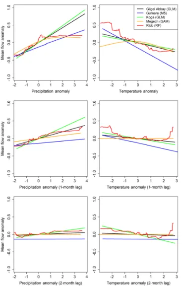
Figure 6. Partial dependence plots for climate covariates in the highest performing model in each basin. Model type is indicated in parentheses.
and inter-model comparisons difficult. However, the partial dependence plots used in the randomForest R package can be developed for any model and provide a mechanism for com-paring the influence that covariates have in the different mod-els and basins (Shortridge et al., 2015). Partial dependence plots were generated for each basin’s best performing model and results are shown for climatic variables in Fig. 6. As ex-pected, models generally respond positively to increases in precipitation and negatively to increases in temperature, with the greatest influence in the current month and decreasing influence at 1 and 2 months prior. The influence of the cur-rent month’s precipitation is linear in three of the five basins; while this is constrained to be the case in the Gilgel Abbay and Koga basins due to the use of a linear model, the lin-ear response in Gumara is not required from the M5 model structure. Interestingly, both Megech and Ribb demonstrate a linear response to negative precipitation anomalies, but little response to positive anomalies. Streamflow response to
tem-Figure 7.Partial dependence plot for agricultural land cover in the highest performing model in each basin. Model type is listed in parentheses for each basin. Dashed lines indicate values that exceed historic levels of agricultural land cover experienced in that basin.
perature is strongest in the Gumara basin; interestingly, this is the basin with the smallest response to precipitation.
The partial dependence plots for the percentage of the basin classified as agricultural land cover indicate a positive relationship between agricultural land cover and streamflow in all basins except for the Gilgel Abbay (Fig. 7). This would be expected if deforestation had contributed to a decrease in evapotranspiration in the contributing watersheds. The exact nature of this response differs across the different rivers, with the relatively minor responses in Koga and Ribb, and much stronger responses in the Gumara and Megech basins. How-ever, this plot also demonstrates some of the limitations asso-ciated with different model structures. The plot for Gumara is highly erratic, indicating that the M5 model might be over-fit to the training data set, despite the use of model averag-ing to reduce model variance. Additionally, the GAM used in the Megech basin was only trained on agricultural land cover values up to 77 %; while this model may be accurately rep-resenting the impact of land cover changes within this range, extrapolating this relationship to higher values leads to pre-dictions that may not be physically realistic.
3.3 Climate change sensitivity and uncertainty assessment
Figure 8.Projected changes in total streamflow (relative to current long-term average) under changing climate conditions. The top two panels show the sensitivity to changes in temperature and precipi-tation when they are varied independently. The bottom panel shows sensitivity to changing temperature in conjunction with decreasing (left panel) and increasing (right panel) precipitation. Dashed lines represent 95 % confidence bounds from bootstrap resampling.
precipitation sensitivity remains relatively constant, even at extreme changes in annual precipitation. The bottom pan-els of the figure show the sensitivity of total inflows to concurrent changes in temperature and precipitation. Un-surprisingly, decreasing precipitation combined with higher temperatures results in greater decreases in total flow than when temperature and precipitation are varied independently. However, even if temperature increases are combined with higher precipitation, total flows decline in the majority of bootstrap resamples.
The uncertainty surrounding temperature sensitivity is a key limitation to using data-driven approaches for climate impact assessment. To better understand which models and basins are contributing to this uncertainty, Fig. 9 shows how the coefficient of variation (the standard deviation of pre-dictions from all bootstrap samples divided by the mean of these predictions) varies as a function of temperature change in each basin. From this figure, it is apparent that the Megech model is by far the largest contributor to model uncertainty; however, it is not clear whether this contribution is due to model structure (the GAM model used for the Megech River) or characteristics associated with the basin itself. To investi-gate how different model structures contributed to this uncer-tainty, the bootstrap resampling procedure was used to assess
Figure 9.Changes in the coefficient of variation across bootstrap resamples from the highest performing model in each basin (left panel) and multiple models all applied to the Gumara basin (right panel).
uncertainty in streamflow predictions in the Gumara River from all model types. This basin was chosen because all six models were able to outperform the climatology model, and thus could be considered good choices for model selec-tion based on predictive accuracy alone. The results indicate that the increase in uncertainty is highest, and increases non-linearly, in the GLM, GAM, and MARS models. Uncertainty increases more slowly in the ANN and M5 models, and no noticeable increase in uncertainty is apparent in the random forest model.
4 Discussion
consis-tently underestimating wet-season flows, resulting in low es-timates of the total annual flow in the rivers. Since multiple reservoirs are planned for construction on these rivers to sup-port irrigation activities, this bias could lead to poor estimates of how much water is available for agricultural use in the short term (i.e., seasonal forecasting) and long term (due to climate change). Interestingly, difficulties in accurately cap-turing high flows have been observed in physical hydrologic models for Ethiopia (e.g., Setegne et al., 2011; Mekonnen et al., 2009) and more generally (e.g., Wilby, 2005). The impli-cations of this limitation should be carefully evaluated before using models for water resource planning or (more impor-tantly) flood risk evaluation.
Depending on the model type used, different mechanisms are available to evaluate covariate importance and influence within the model. This evaluation can be useful in confirm-ing that the model is replicatconfirm-ing relationships between input and output variables in a reasonable manner. While the re-lationships identified in this evaluation are fairly straightfor-ward (for example, increasing runoff with higher precipita-tion and lower temperatures), these simple relaprecipita-tionships are still important in highlighting the mechanisms by which the models make predictions so that they are not “black boxes”. For instance, Han et al. (2007) explore how ANN flood fore-casting models respond to a double-unit input of rain, finding that some formulations respond in a hydrologically meaning-ful way to increased rainfall intensity, while others do not. Similarly, Galelli and Castelletti (2013a) describe how input variable importance can be used to highlight differences in hydrologic processes between an urbanized and forested wa-tershed. The easy manner in which covariate relationships within the GAM and random forest models can be visualized using a single command within their respective R packages is a strong advantage to these approaches compared to meth-ods such as M5 model trees and artificial neural networks. Of course, partial dependence plots can be developed for any model type (as was done in this research), but code must be written by the user and thus requires a higher degree of effort than is necessary for in-package functions. A downside to most machine learning models is that they do not support the statistical formalism in assessing variable importance that is possible when linear models and GAMs are used. However, this formalism often rests on assumptions regarding model residuals that are unlikely to be met in many hydrologic mod-els (Sorooshian and Dracup, 1980).
Within the Lake Tana basin, evaluation of covariate influ-ence indicates that each basin’s model is performing in a reasonable manner, with runoff increasing with higher pre-cipitation levels and decreasing with higher temperatures. The influence of precipitation and temperature is greatest in the current month, and progressively declines to a very small influence after 2 months. This suggests that long-term (multi-month) storage does not significantly contribute to variability in flow volumes. One interesting finding is the non-linear relationship between concurrent month
precipita-tion and runoff that exists in the Megech and Ribb basins, which suggests that above a certain point increasing rainfall does not result in a commensurate increase in streamflow. Other studies have noted the dampening effect that wetlands and floodplains have had on river flows in the region (Dessie et al., 2014; Gebrehiwot et al., 2010); this phenomenon could explain the non-linear relationship identified in this work. The clearly negative relationship between temperature and runoff demonstrates the degree to which upstream evapotran-spiration impacts streamflow and suggests that evapotranspi-ration is largely energy-limited, rather than water-limited. In-creasing agricultural land use appears to be associated with higher runoff in all rivers except for Gilgel Abbay (where no clear relationship between land cover and runoff was ob-served), and suggests that agricultural expansion at the ex-pense of forest cover has reduced the evaporative compo-nent of the water balance in these basins. Finally, the rela-tive performance of different model formulations themselves can also be informative. For instance, the improved perfor-mance of the anomaly-formulation models indicates that the relationship between precipitation and runoff varies through-out the year and could point towards differences in runoff-generating mechanisms in the wet and dry seasons that have been observed in other case studies (Wilby, 2005).
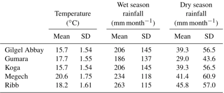
Table 6.Mean and standard deviation values for temperature, wet-season rainfall, and dry-season rainfall in each basin.
Wet season Dry season
Temperature rainfall rainfall
(◦C) (mm month−1) (mm month−1)
Mean SD Mean SD Mean SD
Gilgel Abbay 15.7 1.54 206 145 39.3 56.5
Gumara 17.7 1.55 186 137 29.0 43.6
Koga 15.7 1.54 206 145 39.3 56.5
Megech 20.6 1.75 234 118 41.4 60.9
Ribb 18.2 1.61 263 115 45.8 57.0
hopes for a windfall of additional water to support agricul-ture and hydropower in the region under climate change may be unfounded.
Repeating the climate change sensitivity experiment with multiple models fit to the Gumara watershed indicated that the MARS, GAM, and linear models all result in the largest increase in uncertainty at high temperatures. This indicates that when models are fit to slightly different bootstrap resam-ples of the historic data set, the projected changes in stream-flow at high temperature changes can be highly erratic. This is likely due to the fact that extrapolating the relationships that are observed between historic temperature and stream-flow to higher temperatures can lead to very large changes in streamflow. Fitting the models to bootstrap resamples of the data results in minor changes to these relationships that can result in widely varying projections when the models are used to predict streamflow at higher temperatures, par-ticularly when these relationships are non-linear (as in the GAM). At the other end of the spectrum, the random for-est model exhibits almost no increase in uncertainty at high temperatures, meaning that projections of streamflow at high temperatures are consistent across the bootstrap resamples. This is likely the result of the random forest model structure. The predicted value for each terminal node of a regression tree is the average of all observations that meet the condi-tions described for that node. Thus, the model will not pre-dict values beyond those experienced historically, even if co-variate values exceed those contained within the historic data set. Thus, this model is likely to underestimate the change in streamflow that results from increasing temperatures.
5 Conclusions
In this work, we compared multiple methods for data-driven rainfall–runoff modeling in their ability to simulate stream-flow in five highly seasonal watersheds in the Ethiopian high-lands. Despite the popularity of ANNs in research on stream-flow prediction to date, ANNs were not found to be the most accurate model in any of the five basins evaluated. Other methods, in particular GAMs and random forests, are able to capture non-linear relationships effectively and lend
them-selves to simpler visualization of model structure and co-variate influence, making it easier to gain insights on phys-ical watershed functions and confirm that the model is op-erating in a reasonable manner. However, it is important to carefully evaluate model structure and residuals, as these can contribute to biased estimates of water availability and un-certainty in estimating sensitivity to potential future changes in climate. In particular, autocorrelation in model residuals can result in underestimation of aggregate metrics such as annual flow volumes, even in models with high NSE perfor-mance. Uncertainty in GAM projections was found to rapidly increase at high temperatures, whereas random forest projec-tions may be underestimating the impact of high tempera-tures on river flows. Thorough consideration of this uncer-tainty and bias is important any time that models are used for water planning and management, but especially crucial when using such models to generate insights about future stream-flow levels. By considering multiple model formulations and carefully assessing their predictive accuracy, error structure, and uncertainties, these methods can provide an empirical assessment of watershed behavior and generate useful in-sights for water management and planning. This makes them a valuable complement to physical models, particularly in data-scarce regions with little data available for model pa-rameterization, and warrants additional research into their development and application.
The Supplement related to this article is available online at doi:10.5194/hess-20-2611-2016-supplement.
were performed under NASA Applied Sciences Program grant NNX09AT61G. This research was conducted while S. D. Guikema was affiliated with the Department of Geography and Environ-mental Engineering at Johns Hopkins University. This support is gratefully acknowledged. Any opinions, findings, and conclusions or recommendations expressed in this material are those of the au-thors and do not necessarily reflect the views of the funding sources.
Edited by: D. Mazvimavi
References
Abrahart, R. J. and See, L. M.: Neural network modelling of non-linear hydrological relationships, Hydrol. Earth Syst. Sci., 11, 1563–1579, doi:10.5194/hess-11-1563-2007, 2007.
Achenef, H., Tilahun, A., and Molla, B.: Tana Sub Basin Initial Sce-narios and Indicators Development Report, Tana Sub Basin Or-ganization, Bahir Dar, Ethiopia, 8–9, 2013.
Alemayehu, T., McCartney, M., and Kebede, S.: The water resource implications of planned development in the Lake Tana catchment, Ethiopia, Ecohydrol. Hydrobiol., 10, 211–221, doi:10.2478/v10104-011-0023-6, 2010.
Antar, M. A., Elassiouti, I., and Allam, M. N.: rainfall–runoff modelling using artificial neural networks technique: a Blue Nile catchment case study, Hydrol. Process., 20, 1201–1216, doi:10.1002/hyp.5932, 2006.
Aqil, M., Kita, I., Yano, A., and Nishiyama, S.: Neural Networks for Real Time Catchment Flow Modeling and Prediction, Water Re-sour. Manage., 21, 1781–1796, doi:10.1007/s11269-006-9127-y, 2007.
Asefa, T., Kemblowski, M., McKee, M., and Khalil, A.:
Multi-time scale stream flow predictions: The
sup-port vector machines approach, J. Hydrol., 318, 7–16, doi:10.1016/j.jhydrol.2005.06.001, 2006.
Beven, K. J.: rainfall–runoff Modelling: The Primer, John Wi-ley & Sons, West Sussex, UK, 83–113 and 307–309, 2011. Breiman, L.: Bagging predictors, Mach. Learn., 24, 123–140,
doi:10.1007/BF00058655, 1996.
Breiman, L.: Random forests, Mach. Learn., 45, 5–32, 2001. Chen, F., Mitchell, K., Schaake, J., Xue, Y., Pan, H.-L.,
Ko-ren, V., Duan, Q. Y., Ek, M., and Betts, A.: Modeling of land surface evaporation by four schemes and comparison with FIFE observations, J. Geophys. Res., 101, 7251–7268, doi:10.1029/95JD02165, 1996.
Chibanga, R., Berlamont, J., and Vandewalle, J.: Modelling and forecasting of hydrological variables using artificial neural net-works: the Kafue River sub-basin, Hydrolog. Sci. J., 48, 363– 379, doi:10.1623/hysj.48.3.363.45282, 2003.
Criss, R. E. and Winston, W. E.: Do Nash values have value? Discussion and alternate proposals, Hydrol. Process., 22, 2723– 2725, doi:10.1002/hyp.7072, 2008.
Dessie, M., Verhoest, N. E. C., Admasu, T., Pauwels, V. R. N., Poe-sen, J., Adgo, E., Deckers, J., and NysPoe-sen, J.: Effects of the flood-plain on river discharge into Lake Tana (Ethiopia), J. Hydrol., 519, 699–710, doi:10.1016/j.jhydrol.2014.08.007, 2014. De Vos, N. J. and Rientjes, T. H. M.: Multiobjective training of
ar-tificial neural networks for rainfall–runoff modeling, Water Re-sour. Res., 44, W08434, doi:10.1029/2007WR006734, 2008.
Ek, M. B., Mitchell, K. E., Lin, Y., Rogers, E., Grunmann, P., Ko-ren, V., Gayno, G., and Tarpley, J. D.: Implementation of Noah land surface model advances in the National Centers for Environ-mental Prediction operational mesoscale Eta model, J. Geophys. Res., 108, 8851, doi:10.1029/2002JD003296, 2003.
Elshorbagy, A., Corzo, G., Srinivasulu, S., and Solomatine, D. P.: Experimental investigation of the predictive capabilities of data driven modeling techniques in hydrology – Part 1: Con-cepts and methodology, Hydrol. Earth Syst. Sci., 14, 1931–1941, doi:10.5194/hess-14-1931-2010, 2010a.
Elshorbagy, A., Corzo, G., Srinivasulu, S., and Solomatine, D. P.: Experimental investigation of the predictive capabilities of data driven modeling techniques in hydrology – Part 2: Application, Hydrol. Earth Syst. Sci., 14, 1943–1961, doi:10.5194/hess-14-1943-2010, 2010b.
Friedman, J. H.: Multivariate adaptive regression splines, Ann. Stat., 19, 1–67, 1991.
Galelli, S. and Castelletti, A.: Assessing the predictive capability of randomized tree-based ensembles in streamflow modelling, Hy-drol. Earth Syst. Sci., 17, 2669–2684, doi:10.5194/hess-17-2669-2013, 2013a.
Galelli, S. and Castelletti, A.: Tree-based iterative input variable se-lection for hydrological modeling, Water Resour. Res., 49, 4295– 4310, doi:10.1002/wrcr.20339, 2013b.
Garede, N. M. and Minale, A. S.: Land Use/Cover Dynamics in Ribb Watershed, North Western Ethiopia, J. Nat. Sci. Res., 4, 9– 16, 2014.
Gaume, E. and Gosset, R.: Over-parameterisation, a major obsta-cle to the use of artificial neural networks in hydrology?, Hy-drol. Earth Syst. Sci., 7, 693–706, doi:10.5194/hess-7-693-2003, 2003.
Gebrehiwot, S. G., Taye, A., and Bishop, K.: Forest Cover and Stream Flow in a Headwater of the Blue Nile: Complementing Observational Data Analysis with Community Perception, Am-bio, 39, 284–294, doi:10.1007/s13280-010-0047-y, 2010. Gleick, P. H.: Methods for evaluating the regional hydrologic
impacts of global climatic changes, J. Hydrol., 88, 97–116, doi:10.1016/0022-1694(86)90199-X, 1986.
Han, D., Kwong, T., and Li, S.: Uncertainties in real-time flood forecasting with neural networks, Hydrol. Process., 21, 223–228, doi:10.1002/hyp.6184, 2007.
Harris, I., Jones, P. D., Osborn, T. J., and Lister, D. H.: Up-dated high-resolution grids of monthly climatic observations – the CRU TS3.10 Dataset, Int. J. Climatol., 34, 623–642, doi:10.1002/joc.3711, 2014.
Hastie, T. and Tibshirani, R.: Generalized Additive Models, Stat. Sci., 1, 297–310, 1986.
Hastie, T. and Tibshirani, R.: Generalized additive models, Chap-man and Hall, London, 9–35, 1990.
Hastie, T., Tibshirani, R., and Friedman, J.: The Elements of Statis-tical Learning: Data Mining, Inference and Prediction, 2nd Edn., Springer, New York, 389–414, 2009.
Iorgulescu, I. and Beven, K. J.: Nonparametric direct mapping of rainfall–runoff relationships: An alternative approach to data analysis and modeling?, Water Resour. Res., 40, W08403, doi:10.1029/2004WR003094, 2004.
models, Hydrol. Process., 18, 571–581, doi:10.1002/hyp.5502, 2004.
Kuhn, M.: caret: Classification and regression training, avail-able at: http://CRAN.R-project.org/package=caret, last access: 6 September 2015.
Kuhn, M., Weston, S., Keefer, C., and Coulter, N.: Cubist: Rule- and instance-based regression modeling, available at: http://CRAN. R-project.org/package=Cubist (last access: 6 September 2015), 2014.
Legates, D. R. and McCabe Jr., G. J.: Evaluating the use of “goodness-of-fit” measures in hydrologic and hydroclimatic model validation, Water Resour. Res., 35, 233–241, 1999. Liaw, A. and Wiener, M.: Classification and regression by
random-Forest, R News, 2, 18–22, 2002.
Lin, J.-Y., Cheng, C.-T., and Chau, K.-W.: Using support vector ma-chines for long-term discharge prediction, Hydrolog. Sci. J., 51, 599–612, doi:10.1623/hysj.51.4.599, 2006.
Liston, G. E. and Elder, K.: A Meteorological Distribution System for High-Resolution Terrestrial Modeling (MicroMet), J. Hy-drometeorol., 7, 217–234, doi:10.1175/JHM486.1, 2006. Machado, F., Mine, M., Kaviski, E., and Fill, H.: Monthly rainfall–
runoff modelling using artificial neural networks, Hydrolog. Sci. J., 56, 349–361, doi:10.1080/02626667.2011.559949, 2011. Maier, H. R., Jain, A., Dandy, G. C., and Sudheer, K. P.:
Meth-ods used for the development of neural networks for the pre-diction of water resource variables in river systems: Current sta-tus and future directions, Environ. Model. Softw., 25, 891–909, doi:10.1016/j.envsoft.2010.02.003, 2010.
Mathevet, T., Michel, C., Andreassian, V., and Perrin, C.: A bounded version of the Nash-sutcliffe criterion for better model assessment on large sets of basins, in IAHS-AISH publica-tion, International Association of Hydrological Sciences, 211– 219, available at: http://cat.inist.fr/?aModele=afficheN&cpsidt= 18790113 (last access: 10 February 2016), 2006.
Mekonnen, M. A., Wörman, A., Dargahi, B., and Gebeyehu, A.: Hydrological modelling of Ethiopian catchments using limited data, Hydrol. Process., 23, 3401–3408, doi:10.1002/hyp.7470, 2009.
Milborrow, S.: earth: Multivariate Adaptive Regression Splines, available at: http://CRAN.R-project.org/package=earth, last ac-cess: 6 September 2015.
Montgomery, D. C., Peck, E. A., and Vining, G. G.: Introduction to Linear Regression Analysis, John Wiley & Sons, Hoboken, New Jersey, 84–95, 2012.
Moriasi, D. N., Arnold, J. G., Van Liew, M. W., Bingner, R. L., Harmel, R. D., and Veith, T. L.: Model evaluation guidelines for systematic quantification of accuracy in watershed simulations, T. ASABE, 50, 885–900, 2007.
Nash, J. E. and Sutcliffe, J. V.: River flow forecasting through con-ceptual models part I – A discussion of principles, J. Hydrol., 10, 282–290, doi:10.1016/0022-1694(70)90255-6, 1970.
Pushpalatha, R., Perrin, C., Moine, N. L., and Andréassian, V.: A review of efficiency criteria suitable for evaluat-ing low-flow simulations, J. Hydrol., 420–421, 171–182, doi:10.1016/j.jhydrol.2011.11.055, 2012.
Quinlan, J. R.: Learning with Continuous Classes, in: Proceedings of the 5th Australian Joint Conference on Artificial Intelligence, World Scientific, Singapore, 343–348, 1992.
R Development Core Team: R: A language and environment for sta-tistical computing, R Foundation for Stasta-tistical Computing, Vi-enna, Austria, available at: http://www.R-project.org (last access: 6 September 2015), 2014.
Rientjes, T. H. M., Haile, A. T., Kebede, E., Mannaerts, C. M. M., Habib, E., and Steenhuis, T. S.: Changes in land cover, rain-fall and stream flow in Upper Gilgel Abbay catchment, Blue Nile basin – Ethiopia, Hydrol. Earth Syst. Sci., 15, 1979–1989, doi:10.5194/hess-15-1979-2011, 2011.
Ripley, B. D.: Pattern Recognition and Neural Networks, Cam-bridge University Press, CamCam-bridge, UK, 143–173, 1996. Schaefli, B. and Gupta, H. V.: Do Nash values have value?, Hydrol.
Process., 21, 2075–2080, doi:10.1002/hyp.6825, 2007.
See, L., Solomatine, D., Abrahart, R., and Toth, E.: Hydroinformat-ics: computational intelligence and technological developments in water science applications – Editorial, Hydrolog. Sci. J., 52, 391–396, doi:10.1623/hysj.52.3.391, 2007.
Setegn, S. G., Srinivasan, R., Melesse, A. M., and Dargahi, B.: SWAT model application and prediction uncertainty analysis in the Lake Tana Basin, Ethiopia, Hydrol. Process., 24, 357–367, doi:10.1002/hyp.7457, 2009.
Setegn, S. G., Rayner, D., Melesse, A. M., Dargahi, B., and Srini-vasan, R.: Impact of climate change on the hydroclimatology of Lake Tana Basin, Ethiopia, Water Resour. Res., 47, W04511, doi:10.1029/2010WR009248, 2011.
Sheffield, J., Goteti, G., and Wood, E. F.: Development of a 50-Year High-Resolution Global Dataset of Meteorological Forc-ings for Land Surface Modeling, J. Climate, 19, 3088–3111, doi:10.1175/JCLI3790.1, 2006.
Shortridge, J. E., Falconi, S. M., Zaitchik, B. F., and Guikema, S. D.: Climate, agriculture, and hunger: statistical predic-tion of undernourishment using nonlinear regression and data-mining techniques, J. Appl. Stat., 42, 2367–2390, doi:10.1080/02664763.2015.1032216, 2015.
Solomatine, D. P. and Ostfeld, A.: Data-driven modelling: some past experiences and new approaches, J. Hydroinform., 10, 3– 22, doi:10.2166/hydro.2008.015, 2008.
Sorooshian, S. and Dracup, J. A.: Stochastic parameter estimation procedures for hydrologie rainfall–runoff models: Correlated and heteroscedastic error cases, Water Resour. Res., 16, 430–442, doi:10.1029/WR016i002p00430, 1980.
Steenhuis, T. S., Collick, A. S., Easton, Z. M., Leggesse, E. S., Bayabil, H. K., White, E. D., Awulachew, S. B., Adgo, E., and Ahmed, A. A.: Predicting discharge and sediment for the Abay (Blue Nile) with a simple model, Hydrol. Process., 23, 3728– 3737, doi:10.1002/hyp.7513, 2009.
Sudheer, K. P. and Jain, A.: Explaining the internal behaviour of artificial neural network river flow models, Hydrol. Process., 18, 833–844, doi:10.1002/hyp.5517, 2004.
Van Griensven, A., Ndomba, P., Yalew, S., and Kilonzo, F.: Critical review of SWAT applications in the upper Nile basin countries, Hydrol. Earth Syst. Sci., 16, 3371–3381, doi:10.5194/hess-16-3371-2012, 2012.
Venables, W. N. and Ripley, B. D.: Modern Applied Statistics with S-PLUS, Springer Science & Business Media, New York, 211– 250, 2013.
Wilby, R. L., Abrahart, R. J., and Dawson, C. W.: Detec-tion of conceptual model rainfall–runoff processes inside an artificial neural network, Hydrolog. Sci. J., 48, 163–181, doi:10.1623/hysj.48.2.163.44699, 2003.
Wood, S. N.: Fast stable restricted maximum likelihood and marginal likelihood estimation of semiparametric generalized linear models, J. Roy. Stat. Soc. B, 73, 3–36, doi:10.1111/j.1467-9868.2010.00749.x, 2011.