J. Braz. Soc. Mech. Sci. & Eng. vol.28 número3

Garret N. Vanderplaats

Structural Optimization for Statics,

Dynamics and Beyond

Structural optimization has matured to the point that it can be routinely applied to a wide range of real design tasks. The purpose here is threefold. First, the general optimization task will be defined. Second, the state of the art in structural optimization will be reviewed. Finally, examples will be presented to demonstrate the level of sophistication possible in applying this technology. It is concluded that, while much research always remains, optimization technology has matured to the point where it can and should be used routinely for engineering design.

Keywords: Optimization, structural optimization, automated design

Introduction

With his landmark paper in 1960, Schmit ushered in over forty years of intensive development in structural and general purpose optimization research. This has culminated in numerous commercial products that are available today to solve design problems of remarkable size and complexity. These basic developments, together with modern graphical interfaces, makes it possible to use this technology with very little formal training in optimization theory.1

Despite the widespread availability of this technology, it is seldom taught as a design tool by universities and remarkably underutilized by industry. Yet the motivation to use optimization is compelling. For automobiles, a ten percent mass reduction will increase fuel economy by about seven percent. Only a one percent economy improvement will save nearly three billion dollars per year in the U.S. at the pump. Similarly, by reducing the mass of a commercial aircraft by about two hundred pounds adds a paying passenger for the life of the aircraft. A one pound reduction in the mass of a spacecraft will either add a pound of payload or save about $20,000 per flight to space. The list of examples could continue for pages. Even beyond the cost argument, the savings in natural resources through the use of optimization could be immense.

The purpose here is to briefly review the development of structural optimization leading to the current state of the art and offer examples to demonstrate the power of optimization to enhance the design process

Nomenclature

F = force in member F(X) = objective function gj(X) =j-th inequality constraint hk(X) = k-th equality constraint K = stiffness matrix

l = number of equality constraints L = length of member

m = number of inequality constraints n = number of design variables P = structural load vector S = search direction

U = vector of structural displacements X = vector of design variables X = single design varible

δX = change in design variables

Greek Symbols

Presented at XI DINAME – International Symposium on Dynamic Problems of Mechanics, February 28th - March 4th, 2005, Ouro Preto. MG. Brazil. Paper accepted: June, 2005. Technical Editor: Joé Roberto de França Arruda.

α = move parameter

σ = stress

σ = allowable stress

σijk = stress in element i, component j, load case k

∂ = partial derivative

∇ = gradient operator

Subscripts

i design variable number j inequality constraint number x derivative with respect to x

Superscripts

L lower bound on design variable New new design

Old old design

U upper bound on design variable -1 inverse

What is Design Optimization?

Optimization is intrinsically tied to our desire to excel, whether we are an athlete, artist or engineer. We all adjust some parameters, perhaps our time, to minimize or maximize one or more results such as income, leisure time or job satisfaction. We do this subject to limitations or constraints, such as physical ability, time available, legal restrictions or moral codes of conduct. Thus, whatever our field of endeavor, we constantly strive to solve a constrained optimization problem.

In engineering, we create products. To do this, we normally use computer analysis to judge the quality of our designs. We use computational fluid dynamics codes to calculate energy requirements and flow patterns in a ducting system. We use finite element analysis to calculate stresses, deflections, vibration frequencies, etc. of a structure. In almost all disciplines, we use computational, and sometimes experimental, tools to judge the quality of our proposed designs. If not satisfactory, we modify the design and perform repeated analyses in an effort to improve the product, or at least meet the design requirements.

This traditional approach of analyze and revise normally involves only changing a few variables (often only one) at a time and does not account very well for the interaction among the variables.

Now imagine we can change large numbers of design parameters simultaneously in order to improve the design while satisfying all design requirements, at the same time accounting for the interactions among the parameters. This is exactly what numerical optimization does.

called an objective function which we wish to minimize or maximize. Other outputs may be required to be within some bounds. These we call constraints. Both the objective(s) and constraints are functions of the input or design variables contained in X.

Numerical optimization solves the general problem: Find the values of the design variables contained in X that will;

Minimize

( )

F (1)

Subject to:

( ) 0 1,

g X j m

j ≤ = ₍₂₎

1,

L U

i i i

X ≤X ≤X i= n (3)

The function, F(X) is referred to as the objective or merit function and is dependent on the values of the design variables, X, which themselves include member dimensions or shape variables of a structure as examples. The limits on the design variables, given in Eq. (3), are referred to as side constraints and are used simply to limit the region of search for the optimum. For example, it would not make sense to allow the thickness of a structural element to take on a negative value. Thus, the lower bounds are set to a reasonable minimum gage size. If we wish to maximize F(X), for example, maximize fuel economy, we simply minimize the negative of F(X).

The gj(X) are referred to as constraints, and they provide bounds on various response quantities. A common constraint is the limits imposed on stresses at various points within a structure. Then if

σ

1 0

ijk

σ

σ − ≤ (4)

where i = element j = stress component k= load condition

Additionally, we could include equality constraints of the form

( ) 0 1,

k

h X = k= l (5)

Normally, equality constraints can be included in the original problem definition as two equal and opposite inequality constraints.

Now consider how we might solve this general optimization problem. One approach would be to pick many combinations of the design variables and call our analysis program to evaluate each, picking the one with the best objective function which also satisfies all constraints. This would be a classical random search approach or perhaps the modern version known as genetic search (Hajela, 1990).

Another approach would be to perturb each design variable and evaluate the objective and constraint functions. This would determine the sensitivity (gradient) of the design with respect to the variables. With this information, we can mathematically (numerically) determine how to change the design variables to improve the objective while satisfying the constraints. There are a multitude of such “gradient based” methods and considerable software available today (Vanderplaats, 2004a).

These methods closely model what we do in design already. Normally, we begin with a candidate design and ask “How can we change the design to improve it?” Thus, we modify our design as;

New Old

X =X +δX (6)

Optimization does much the same thing, but in two steps. First, we ask what direction to move in and then we ask how far to move. That is,

New Old

X =X +αS (7)

where S is the search direction and α is the number of steps we move in this direction (partial steps are allowed).

The difference in optimization algorithms is mainly in how we calculate the search direction, S, and how we do the “one-dimensional search” to determine α. The key point here is that all variables are considered simultaneously according to their effect on the objective function and all constraints. Also, since this is all automated and today’s computers are very fast, we can find an optimum design with much less time and effort than just finding an acceptable design using traditional methods.

This problem statement provides a remarkably general design approach and a multitude of methods are available today for solving this general problem. Much of the theoretical development has been in the operations research community and applications there are widespread today. In engineering, while development has been underway for over forty years, applications have lagged far behind. The time has come for that to change.

Optimization History

Structural optimization dates to the work of Maxwell(1869) and Mitchell (1904). The modern, computer based, era of structural optimization was ushered in by Schmit’s classical paper in 1960, though in his 1981 review of Structural Synthesis development, he credits a paper by Klein (1955) for providing some key ideas.

Here, we will briefly offer a narrative of the development of general optimization algorithms followed by development of structural optimization. The distinction is that general optimization provides the actual optimization algorithm while structural optimization offers advanced methods for making the best use of these algorithms. Most of these details may be found in Vanderplaats (2004a).

Optimization Algorithms

During the 1950s and early 1960s, random search methods were popular, where the components of the X vector were chosen randomly, an analysis was performed and if an improved design was found, it was kept. This was repeated until no progress could be made or computer resources were exhausted (the usual case). The choice of random values could be the actual values of Xi or perturbations of these values. Some researchers observed that, after some time, they could create a vector from the worst to the best design and accelerate the process by moving in this direction. One might observe that this is a (rather poor) gradient search. These methods are easy to program but are very inefficient and are limited to only a few variables.

Focus during the 1960s included Sequential Linear Programming (Kelly, 1960) (SLP), Sequential Unconstrained Minimization Techniques (Fiacco and McCormick, 1968) (SUMT) and Feasible Directions methods (Zoutendijk, 1960). Though some non-gradient based methods were also developed during this period, these gradient based methods were generally considered to be more efficient and reliable.

algorithm that will drive the design to a Kuhn-Tucker point, improved efficiency and robustness will result. During the late 1970s, development of response surface methods began (Vanderplaats, 1979 and Myers and Montgomery, 1995) and has continued since.

The 1980s were a period of refinement ending with renewed interest in random methods in the engineering community and Sequential Unconstrained Minimization Techniques by the operations research community. The random (and related) methods include Genetic Search (Hajela, 1990), Simulated Annealing (Nemhauser and Wolsey, 1988) and related methods that attempt to mimic natural evolutionary processes. The Sequential Unconstrained Minimization Techniques focused on interior point methods based on the Kuhn-Tucker conditions (Hagar, et al, 1994). Throughout the 1990s, Genetic Search algorithms were the focus of considerable research by the engineering community and a new method called Particle Swarming was added (Venter and Sobieszczanski-Sobieski, 2003). Meanwhile, the operations research community focused on interior point methods and continued to refine these. For engineering problems, an exterior penalty function method was developed for solution of very large scale continuous and discrete variable problems (Vanderplaats, 2004b).

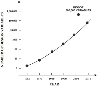
As optimization algorithms have improved, the size and complexity of the engineering applications has grown. Figure 1 shows the trend in engineering problem size beginning in 1960. While there is considerable scatter in the data to create this figure, it is seen that there has been an exponential growth in problem size.

N

U

M

B

E

R

O

F

D

E

S

IG

N

V

A

R

IA

B

L

E

S

BIGDOT 500,000 VARIABLES

Figure 1. Growth in optimization problem size.

Structural Optimization

Structural optimization began in earnest with Schmit’s classical paper (1960). This ushered in the era of numerical search methods which were more general than previous analytically based methods such as Shanley’s work (1952). The 1960s saw a great deal of research in structural optimization, dealing mainly with member sizing of trusses, frames and shell structures. Initially, gradients were calculated by finite difference methods. It was not until 1965 that gradients were calculated analytically and this happened with such little fanfare that the original published work by Fox (1965) on calculating gradients analytically is relatively unknown and seldom referenced.

Gradients of displacements are calculated from the basic finite element analyses equations,

Ku=P (8)

where K is the master stiffness matrix, P is the vector of applied loads and u is the vector of displacements.

Differentiating with respect to design variable Xi and rearranging gives

1

i i i

u P K

K u

X X X

−  

∂ ₌ ∂ ₋∂

 

∂ ∂ ∂ 

(9)

Because the stiffness matrix has already been decomposed, this is a simple and efficient calculation. From this the derivatives of stresses are calculated from the stress recovery equations. Derivatives of eigenvalues and eigenvectors, as well as various other responses are calculated in a similar fashion.

By the end of the 1960s it was becoming apparent that numerical optimization was limited to perhaps fifty variables and was computationally too expensive to the a usable design tool. This was particularly emphasized in a paper by Gallatly, Berke and Gibson (1971) when they called the 1960s “the period of triumph and tragedy” for structural optimization. Thus, the 1970s began the era of optimality criteria methods. Optimality criteria offered the ability to deal with large numbers of design variables but with a limited number of constraints and without the generality of numerical optimization methods. Numerical optimization methods were given new life in 1974 when Schmit and Farshi (1974) published their work on approximation concepts. These methods were based on the concept of creating approximations using the underlying physics to allow for large moves and this reduced the number of detailed finite element analyses from well over 100 to the order of ten. For statically determinate trusses or membrane structures, these approximations were shown to be exact for stress and displacement constraints. Parallel to the development of approximation concepts, the adjoint method for gradient computations was developed (Arora and Haug, 1979 and Vanderplaats, 1980). Finally, in the late 1970s Fleury and Sanders (1977) reconciled numerical optimization and optimality criteria methods by showing that optimality criteria are closely related to duality theory in numerical optimization.

For a detailed understanding of the development and state of the art at the end of the 1970s, Schmit’s AIAA History of Key Technologies (1981) paper is an excellent resource.

The 1980s were a period of refinement and the initial steps of creating commercial structural optimization software. Second generation approximations were created using force approximations (Bofang and Zhanmei, 1981 and Vanderplaats and Selajegheh, 1989)instead of the earlier stress approximations. Similarly, Releigh quotient approximations were created for eigenvalue constraints (Canfield, 1990). These new approximations expanded the element types to shell and frame elements among others. Importantly, for such elements as frames it was now possible to treat the physical dimensions as design variables and section properties as intermediate variables so that the designer could now deal with the actual variables of interest.

P A

Figure 2. Simple rod.

Minimize

XL (10)

Subject to;

F X

σ= ≤σ

(11)

Note that the objective is linear but the constraint is nonlinear. We could linearize both and repeatedly solve the problem using this approximation. Such an approach is just sequential linear programming and is generally not very reliable or efficient.

Now consider a change in variables so X = 1/A. The problem is now

Minimize

L

X (12)

Subject to;

FX

σ= ≤σ (13)

We’ve now converted the problem to one with a linear objective and a nonlinear constraint to one with a nonlinear objective with a linear constraint. Such a problem is better conditioned for optimization. Furthermore, we can create a linear approximation to the constraint and keep the original objective, since it is easily calculated, along with its derivatives.

That is,

0

X X

σ σ

σ

δ

This approach was offered by Schmit and Farshi (1974) in the 1970s and this allowed us to solve structural optimization problems of rods and membranes with an order of magnitude improvement in efficiency.

In the 1980s, Bofang (1981), and Vanderplaats and Selajeghgh (1989) proposed approximating the force on the elements instead of approximating the stress.

Thus,

0

A

F F A

A

δ σ≈ + ∇ •

(15)

This is actually a higher order approximation and is also applicable to elements other than rods and membranes.

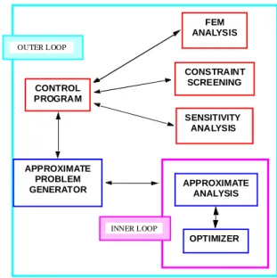
Figure 3 shows the organization of a modern structural optimization program. The general approach is to first perform an analysis and evaluate all constraints. These are then screened to eliminate, temporarily, those that are not critical or near critical. Then, the sensitivity analysis is performed. The approximate problem is then generated and solved. The key points are that the approximations are based on physics and are of very high quality and that the optimizer never actually calls the finite element analysis. The result is that optimization normally requires only 10 or so detailed finite element analyses to achieve an optimum, even when there are very large numbers of design variables and constraints.

CONTROL PROGRAM

SENSITIVITY ANALYSIS

OPTIMIZER APPROXIMATE

PROBLEM

GENERATOR APPROXIMATE_ANALYSIS FEM ANALYSIS

CONSTRAINT SCREENING

INNER LOOP OUTER LOOP

Figure 3. Modern structural optimization.

In recent years, topology optimization has become popular. Here, given a design volume filled with material, the objective is to find the stiffest structure using a specified fraction of the material. This is a powerful tool for defining an initial structure for later refinement using shape and sizing optimization.

Optimization in a Commercial Environment

Although some commercial optimization capabilities were developed in the early years, the serious commercialization of this technology began in the late 1980s and began to proliferate in the 1990s and today. Commercial software generally falls into two distinct categories; general purpose optimization and fully integrated finite element based structural optimization. With few exceptions there has not been a significant effort to “tightly couple” optimization with other disciplines such as computational fluid mechanics.

Due to the nature of optimization algorithms and their implementation, the capabilities and features of the various offerings can differ greatly so some effort is needed to choose the best software for a particular group or company. Most vendors take considerable effort to create “user friendly” software so the user does not need to be an expert in optimization theory.

Examples

optimization software. Most problems solved in a purely research environment are not sophisticated enough to be useful here and most real commercial problems are proprietary and cannot be published. Therefore, these examples fall somewhere between academic and real commercial products. The linear analysis based structural optimization examples are solved by GENESIS.

Shape Optimization of a Pin

Figure 4 shows a cutaway of a symmetric structure with a load on the steel pin. The outer structure is ceramic and the intermediate portion is an adhesive. The objective is to change the shape of the outer structure to minimize the maximum stress with deformation limits. This is a nonlinear contact problem solved by coupling the ABAQUS analysis software with the VisualDOC general purpose optimization software. Nine shape variables were used and the maximum stress was reduced by eleven percent. This is typical of the improvement optimization provides for an existing design. The nonlinear codes, such as ABAQUS, LS-Dyna, PamCrash, etc. to not use the high quality approximations available for linear analysis based optimization so this coupling of the analysis with a general purpose optimizer is the typical approach. This is a perfectly valid optimization approach and the only negative is that it requires many more analyses than for the linear case. This is alleviated somewhat by parallel processing but is still relatively expensive. Using this approach, we can solve nonlinear contact problems such as this, crash energy absorption, air bag deployment optimization and airfoil optimization, as examples.

Figure 4. Shape optimization.

Car Body Reinforcement

As noted above, structural optimization is more advanced than general purpose optimization because we can calculate gradients of the needed responses and because we have very high quality approximation techniques to provide efficiency and reliability.

Figure 5 shows a car body model which we wish to reinforce to increase the bending and/or torsion frequency. The approach used here was to allow every element in the model to be optimized for thickness (with a lower bound of the original design) with the constraint that only a specified fraction of the material may be used. Here, 34,560 sizing variables were used. While somewhat difficult to see in Figure 5 (unless viewed in color), reinforcement was added in the areas of the firewall, rocker panels and rear fender areas.

Table 1 gives the increase in bending or torsion frequency for different values of added mass.

Figure 5. Car body reinforcement.

Table 1. Frequency increases. Increased Frequency (Hz) Added

Mass (Kg) Maximize First Torsion Frequency

Maximize First Bending Frequency

2.64 4.81 6.42

7.32 7.56 9.89

15.06 9.66 11.22

Topology Optimization of a Simple Support

Figure 6 shows topology optimization of a simple support. This was a 100,000 variable example where the density of each element was designed and the strain energy of the structure was minimized. The key feature here is that manufacturing constraints were imposed to insure that the part could be cast.

Initial Design Final Design

Figure 6. Support.

Topology Optimization Without Manufacturing Constraints

If topology optimization is performed without considering manufacturing issues, very attractive structures are often produced but these cannot be easily manufactured. Figure 7 is such an example where just over one million design variables were used. This structure was optimized to minimize strain energy under the applied load.

Initial Design

Final Design

Figure 7. Skeletal support.

Matching Modal Frequencies

An aerospace application is to design a fin such as that shown in Fig. 8 to match desired frequencies. This may occur when a vibration test is performed and it is desired to adjust the finite element model to match the measured values. Figure 8 shows an example of a typical missile fin. Here, the thickness of the solid fin was designed to give a first frequency of 5Hz +0.2Hz and a second frequency greater than 12Hz. Additionally, stress and displacement constraints were imposed and it was required to minimize the mass. There were a total of 144 design variables and the mass was reduced 39% while satisfying the stress and displacement constraints. The first frequency was moved from 3.37Hz to 5.18Hz and the second frequency was moved from 8.61Hz to 12.04Hz.

Uniform Thickness Airfoil

Optimized Airfoil Uniform Thickness

Airfoil

Optimized Airfoil

Figure 8. Matching frequencies.

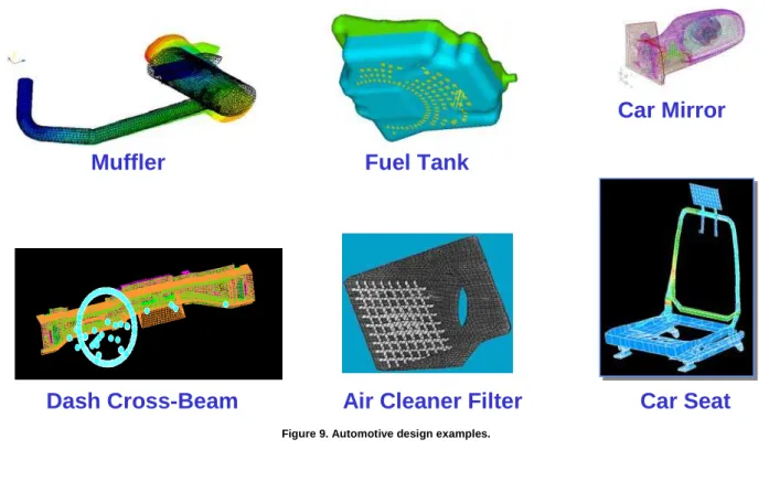
Various Automotive Design Examples

Figure 9 shows various applications in the automotive industry. These are actual design examples and so details are proprietary. However, it is clear that real structures can be efficiently designed with optimization. In some cases, special features need to be added to the software to achieve reasonable results. For example, the fuel tank was stiffened by adding the indentations (beads) to the bottom. If the optimization software had been used without consideration of the real design conditions, an unreasonable design would have resulted. This is because the stiffest design would be one with much different but stiffer indentations but at the cost of greatly reducing fuel capacity. The solution was to create “volume” elements inside the tank and constraining this volume to be the required capacity.

Car Mirror

Fuel Tank

Muffler

Air Cleaner Filter

Car Seat

Dash Cross-Beam

Heat Shield Optimization

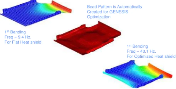
Figure 10 shows a heat shield where it is desired to add a bead pattern in order to increase the first bending frequency without increasing the mass. The initial design has a frequency of 9.4 Hz. By automatically designing the bead pattern, the frequency was increased to 40.1 Hz.

1st_Bending Freq = 9.4 Hz. For Flat Heat shield

Bead Pattern is Automatically Created for GENESIS Optimization

1st_Bending Freq = 40.1 Hz. For Optimized Heat shield

Figure 10. Heat shield optimization.

Summary

A narrative of the development of optimization leading to the current use of this technology in industry has been offered. Development of this technology has followed two distinct tracks. One is optimization algorithms for general applications and the other is special techniques for structural optimization. The distinction is that structural optimization methods create a high quality approximation based on physics (as opposed to simple linearization) to improve efficiency and robustness and then uses a general purpose optimizer to solve this approximate problem.

Commercial software is available for both classes of problems. This software is highly refined and can be used with very limited knowledge of optimization theory.

Finally, a variety of applications have been presented to demonstrate the power available today. It is noted that some of these examples are not actual commercial applications because those are usually proprietary. Indeed, to the best of this author’s knowledge, the largest structural sizing optimization problem solved in industry exceeds 250,000 design variables with topology optimization problems exceeding two million variables.

It is concluded that the state of the art is well refined and is readily available in the commercial environment to improve design quality, reduce design time and increase corporate profits. Indeed, it is argued that no computational technology today is as effective as an advanced design tool as is numerical optimization.

References

ABAQUS Users Manual, 2004, Version 6.4, Abaqus, Inc., Patucket, RI.

AFT Mercury 5.0 User's Guide, 2001, “Applied Flow Technology”,

Woodland Park, Colorado.

Arora, J. S. and Haug, E. J., 1979, “Methods of Design Sensitivity

Analysis in Structural Optimization,” AIAA Journal, Vol. 17, pp. 970-974.

Bofang, Z. and Zhanmei, L., 1981,”Optimization of Double-Curvature

Arch Dams” (In Chinese), Chinese Journal of Hydraulic Engineering, No. 2,

pp. 11-21.

Canfield, R. A., 1990, “High-Quality Approximations of Eigenvalues in Structural Optimization”, AIAA J., Vol. 28 No. 6, pp. 1116-1122.

Cressie, N., 1991, “Statistics for Spatial Data”, John Wiley and Sons,

Inc., New York, NY, pp. 1-26.

Fiacco, A. V., and G. P. McCormick, 1968, “Nonlinear Programming:

Sequential Unconstrained Minimization Techniques”, John Wiley and Sons,

New York.

Fleury, C. and Sanders, G., 1977, “Relations Between Optimality Criteria and Mathematical Programming in Structural Optimization,”

Proceedings of the Symposium on Applications of Computer Methods in Engineering, University of California, Los Angeles, pp. 507-520.

FLUENT 5 User's Guide, 1998, FLUENT, Inc., Lebanon, NH. FLUX2D User’s Manual, 2001, CEDRAT Corporation, Meylan, France. Fox, R. L., 1965, “Constraint Surface Normals for Structural Synthesis

Techniques,” AIAA Journal, Vol. 3, No. 8, pp. 1517-1518.

Gabriel, G. A., and Ragsdell, K. M., 1977, “The Generalized Reduced

Gradient Method: A Reliable Tool for Optimal Design,” ASME J. Engin.

Ind., Series B, Vol. 99, No. 2, pp. 394-400.

Gallatly, R. A., Berke, L. and Gibson, W., 1971, “The Use of Optimality

Criteria in Automated Structural Design,” presented at the 3rd _{Conference on}

Matrix Methods in Structural Mechanics, Wright-Patterson Air Force Base, Ohio.

Garcelon, J., Wipke, K. and Markel, T., 2000, “Hybrid Vehicle Design

Optimization,” AIAA paper No. 2000-4745, Proc. 8th AIAA/

USAF/NASA/ISSMO Symposium on Multidisciplinary Analysis and Optimization, Long Beach, CA, Sept. 6-8.

GENESIS User’s Manual, 2004, Version 7.5: Vanderplaats Research &

Development, Inc., Colorado Springs, CO.

Hager, W.W., D. W. Hearn and P. M. Pardalos, 1994, “Large Scale

Optimization; State of the Art,” Kluwer Academic Publishers, pp. 45-67.

Hajela, G., 1990, “Genetic Search – An Approach to the Nonconvex Optimization Problem,” AIAA Journal, Vol. 26, No. 7, pp. 1205-1210.

Kelley, J. E., 1960, “The Cutting Plane Method for Solving Convex

Programs,” J. SIAM, Vol. 8, pp. 702-712.

Klein, B., 1955, “Direct use of Extremal Principles in Solving Certain

Optimization Problems Involving Inequalities,” Journal of the Operations

Research Society of America, Vol. 3, pp. 168-175.

Maxwell, C., 1869, Scientific Papers, Vol. 2, Dover Publications, New

York, 1952, pp. 175-177.

Mitchell, A. G. M., 1904, “The Limits of Economy of Material in Frame Structures,” Philosophical Magazine, Series 6, Vol. 8, No. 47, pp. 589-597.

Myers, R. H. and Montgomery, D. C., 1995, Response Surface

Methodology, John Wiley & Sons, NY.

Nemhauser, G. L. and Wolsey, L. A., 1988, “Integer and Combinatorial Optimization”, Chapter 3 , John Wiley & Sons.

Rockafellar, R. T., 1973, “The Multiplier Method of Hestines and

Powell Applied to Convex Programming,” J. Optim. Theory Appl., Vol. 12,

No. 6, pp. 555-562.

Shanley, R. R., 1952, “Weight-Strength Analysis of Aircraft Structures”, McGraw Hill, New York.

Schmit, L.A., 1960, “Structural Design by Systematic Synthesis,”

Proceedings, 2nd Conference on Electronic Computation, ASCE, New York, pp. 105-132.

Schmit, L. A. and Farshi, B., 1974, “Some Approximation Concepts for

Structural Synthesis,” AIAA Journal, Vol. 12, pp. 692-699.

Schmit, L. A., 1981, “Structural Synthesis – Its Genesis and

Development,” AIAA Journal, Vol. 19, No. 10, pp. 1249-1263.

Vanderplaats, G. N., 1979, “An Efficient Algorithm for Numerical

Air-foil Optimization,” AIAA J. Aircraft, Vol. 16, No. 12.

Vanderplaats, G. N., 1980, “Comment on ‘Methods of Design

Sensitivity Analysis in Structural Optimization’,” AIAA Journal, Vol. 18, pp.

1406-1407.

Vanderplaats, G. N. and Salajegheh, E., 1989, “A New Approximation

Method for Stress Constraints in Structural Synthesis,” AIAA J., Vol. 27 No.

3, pp. 352-358.

Vanderplaats, G. N., 2004a, “Numerical Optimization Techniques for

Engineering Design - With Applications”, 4th. Edition, Vanderplaats

Research & Development, Inc., Colorado Springs, CO.

Vanderplaats, G. N., 2004b, “Very Large Scale Continuous and Discrete

Variable Optimization,” Proc. 10th _{AIAA/ISSMO Multidisciplinary Analysis}

and Optimization Conference, Paper No. AIAA-2004-4458, 30 Aug. – 1 Albany, NY.

Venter, G. and Sobieszczanski-Sobieski, J., 2003, “Particle Swarm

Optimization,” AIAA Journal, Vol. 41 No. 8, pp. 1583-1589.

VisualDOC User’s Manual, 2004, Version 5.0: Vanderplaats Research & Development, Inc., Colorado Springs, CO.

Zoutendijk, G., 1960, “Methods of Feasible Directions”, Elsevier,