Eduardo A. Tannuri
and Leonardo K. Kubota
[email protected] Depart. of Naval Architecture and Ocean Eng
Celso P. Pesce
Depart. of Mechanical Engineering Escola Politécnica, University of São Paulo Av. Prof. Mello Moraes, 2231 05508-900 Cidade Universitária, São Paul. Brazil [email protected]
Adaptive Techniques Applied to
Offshore Dynamic Positioning
Systems
Dynamic positioning systems (DPS) comprise the deployment of active propulsion to maintain the position and heading of a vessel. Several sensors are used to measure the actual position of the floating body, while a control algorithm is responsible for the calculation of forces to be delivered by each propeller, in order to counteract all environmental forces, such as wind, waves and current loads. The controller cannot directly compensate motions in the sea waves frequency range, since they would require an enormous amount of power to be attenuated, possibly causing damage to the propeller system. That is the reason why a filtering algorithm is to be put in place to separate high-frequency components from the low-high-frequency ones, which are, then, fed into the control loop. Usual commercial systems apply Kalman filtering technique to perform such task, due to the smaller phase-lag introduced in the control loop compared to conventional low-pass filters. The Kalman filter draws on a model of the system to be controlled, which, in turn, depends on an unknown parameter, related to the wave frequency. Adaptive filtering is called upon with a view to perform an on-line estimation of such parameter. Most control algorithms, however, rely on fixed gains, thus making it possible for a noticeable performance degradation to take place in some situations, as those associated to mass variation during a loading operation. This paper presents the application of model-reference adaptive control (MRAC) technique to DPS’s, cascaded with the commonly used adaptive Kalman filter. The model of a dynamically-positioned shuttle tanker exposed to waves and current is employed to highlight the advantages of the adaptive controller compared to commonplace fixed-gain controllers.
Keywords: Adaptive control, dynamic positioning system, Kalman filter
Introduction
Dynamic Positioning Systems (DPS) are defined as a set of components used to keep a floating vessel on a specific position or on a desired path through the action of propellers. DPS includes position and heading measurement systems, a set of control algorithms and propellers. Several offshore operations are carried out using DPS, such as drilling a sub sea petroleum well, underwater pipe-laying, offloading and diving support.1
The environmental forces acting on a floating vessel are complex, and induce at least two distinct kinds of motions. Sea waves consist of a large number of oscillatory components, with several directions, amplitudes and phases. The resulting energy spectrum has a peak value between 0.3rad/s and 1.3rad/s. Wind-generated waves give rise to large oscillatory forces and moments on a vessel, inducing high-frequency motions (in the same frequency range of waves). Additionally, environmental loads include slowly-varying disturbances caused by wind, current and wave-drift forces, which induce low-frequency oscillations and steady motions on vessels. DPS must suppress the low-frequency motions, keeping the mean position of the vessel as close as possible to the desired point. High-frequency motions, however, are difficult to be handled by the control system, since they would require an enormous amount of power to be attenuated, leading to extra fuel-consumption and increased rate of propellers wear-out, due to thruster modulation (high frequency oscillations in propellers).
Therefore, a sophisticated filtering algorithm must be included in the control loop. The purpose of the wave filter is to separate the high-frequency oscillatory wave induced motion from the motion caused by slowly varying disturbances. Feedback control action must be implemented using the filtered low-frequency vessel dynamics, enabling thruster modulation and all related problems to
Presented at XI DINAME – International Symposium on Dynamic Problems of Mechanics, February 28th - March 4th, 2005, Ouro Preto. MG. Brazil. Paper accepted: June, 2005. Technical Editor: José Roberto de França Arruda.
be avoided. Of course, the introduction of a wave filter in the control loop leads to increased phase-shift (time lag) and to a lower stiffness (reaction to variations in input variables and disturbances). So, a good filter is the one that keeps the modulation below tolerable limits while retaining maximum system stiffness. Earlier DPS used conventional Butterworth low-pass wave filters or notch filters, which could be easily implemented in analog circuits (Fossen, 1994). However, the main disadvantage of such filters is the introduction of additional phase-lag, causing poor performance, increased oscillations and, sometimes, instability in closed-loop response.
An alternative to conventional filtering is to apply observer-based techniques, such as Kalman filtering. One of the main characteristics of Kalman filter is the use of available information regarding the dynamical behavior of the process. The vessel motion due to slow disturbances and due to wave action is modeled. The motion information (predicted by the filter model) is combined with available observations, and an optimum state estimator is then constructed. The vessel motion is regarded as the sum of two linearly-independent response functions. A low frequency model yields motions due to maneuvering forces and environmental forces due to wind, current and wave drift, and a high-frequency model yields vessel response due to waves. The idea of separating the filter model into a low and a high-frequency model was originally suggested by Balchen et al. (1976).
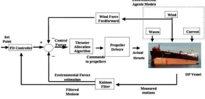
The control algorithm itself calculates thrust forces and moment based on low-frequency motion. Modern commercial systems still employ simple PD algorithms. The integral action is accounted for thanks to the direct compensation of environmental forces, which are also estimated by the Kalman filter, as will be shown in the next section. A simplified block diagram of a DP System is presented in Fig.1.
Figure 1. DP System block diagram.
The robustness and simplicity of PD controller are the main reasons for its widespread utilization. Furthermore, it satisfies the performance requirements of a great number of DP ships. Tuning of the controller gains is normally carried out during the DPS installation, and sometimes requires the execution of some maneuvers in order to evaluate ship overall dynamics and maneuverability (Bray, 1998).
However, during harsh environmental conditions, the system may display loss of performance, since the PD gains were adjusted under a calm sea state, as described in Bray (1998). Furthermore, in some offshore operations, oil is transferred from one moored FPSO or platform to a DPS shuttle tanker. This operation can last as long as 24h, and the mass of the tanker may undergo a threefold increase in its original value, thus imparting a substantial change in the tanker dynamic properties. In this case, a fixed-gain controller would hardly prove a fitting approach, since it would require full attention on the part of the operator, who, in turn, must perform manual corrections in the positioning of the tanker, in order to keep said vessel within a safe distance away from the FPSO.
Therefore, constant-gain PD controller is not appropriate for ships that must operate under a wide “environmental window” or for ships undergoing significant mass variation throughout the operation. Such and other reasons have led researchers to apply different control methodologies to the DPS. All initiatives feature advantages when compared to the fixed-gain PD controller, demonstrated by means of experiments or simulations. However, the academic community was not able to sway operators and manufacturers, who still rely on PD controller. Some examples of such novel controllers may be found in Katebi et al. (1997), Aarset et al. (1998) and Tannuri et al. (2001).
In the present paper, the problems associated to the PD controller are solved by means of a model-reference adaptive controller. It is shown that the overall structure of the PD controller is still preserved, and the adaptive algorithm is responsible for the on-line correction of control gains. With the present solution, the authors try to address the problem, while retaining the simplicity of the PD controller, which is one of the main reasons for its widespread utilization.
The controller is developed and tested on the ship model for only one degree of freedom. Simulations are carried out considering a shuttle tanker similar to the vessels operating in Brazilian waters.
Nomenclature
â =estimated parameters vector ã =vector of parameter estimation error
c = damping in degree of freedom model, N/m/s or N/rad/s C = damping matrix
D =derivative gain e =tracking error
K = stiffness in degree of freedom model, N/m or N/rad FiE = environmental loads, N or N.m
FiT = forces and moment by the propulsion system, N or N.m FE = vector with environmental loads
FT = vector with thrusters forces and moment vector
G =matrix associated with Lyapunov function
Iz = moment of inertia of the vessel about the vertical axis K = Kalman gain matrix
m = total mass in degree of freedom model, kg or kg.m2 M = vessel mass matrix
M = vessel mass, kg
M11 =surge added mass, kg
M22 =sway added mass, kg
M66 = yaw added mass, kg.m2
M26 = sway-yaw added mass, kg.m
P = estimate of cov(Ψ [k]).
Pii = power spectrum of ship motion i, m2/rad/s or rad2/rad/s
PR = proportional gain
QC = matrix associated with control law gains QFL= covariance matrix of L
ω
F
QH =covariance matrix of H
ω
QL =covariance matrix of L
ω
R=covariance matrix of v
RAOi =Response Amplitude Operator, dimensionless or rad/m
S = power spectrum of wave surface height, m2/rad/s
u = control signal
uc = reference signal
v = vector of measurement white noises V = Lyapunov function
x = a priori estimate vector
xˆ = a posterior estimate vector
i
xɺ = midship absolute velocities, m/s or rad/s
xH = vector with high frequency states
xL = vector with low frequency states,
X,Y =Position of vessel center point in absolute reference frame, m
x =error state vector
ym =position of the reference model
z = vector with measred signals Greek Symbols
β = wave incidence angle related to the ship, rad
β0,β1 = positive coefficients of a stable (Hurwitz) polynomial
∆t = sampling time, s ε = innovation
λ = the forgetting factor Γ
Γ Γ
Γ = = = = matrix associated with control gains ω = wave frequency, rad/s
0
ω
= peak frequency of high frequency motion (rad/s)FL
ω
= vector of white noises in environmental forces model
H
ω
= vector of white noises in low frequency model
L
ω
= vector of white noises in low frequency model Ψ = vessel heading, rad
ζ = relative damping ratio of high frequency motions Subscripts
1 relative to surge motion 2 relative to sway motion 6 relative to yaw motion
E relative to environmental agents
H relative to high frequency motion
L relative to low frequency motion
M relative to the reference model
T relative to propulsion system
System Modeling
The following dynamic model governs the low frequency horizontal motions of a vessel:
(
) (
)
(
)
(
)
(
)
.; ;
6 6 6 1 26 2 26 6 66
2 2 6 1 11 6
26 2 22
1 1 2 6 26 6 2 22 1
11
T E Z
T E
T E
F F x x M x M x M I
F F x x M M x M x M M
F F x M x x M M x M M
+ = +
+ +
+ = +
+ + +
+ = − +
− +
ɺ ɺ ɺ ɺ ɺ ɺ
ɺ ɺ ɺ
ɺ ɺ ɺ
ɺ ɺ ɺ ɺ
ɺ
(1)
where Iz is the moment of inertia about the vertical axis; M is vessel
mass, Mij are added mass matrix terms, F1E, F2E, F6E are surge, sway
and yaw environmental loads (current, wind and waves) and
T T
T F F
F1 , 2 , 6 are forces and moment delivered by the propulsion
system. The variablesxɺ1, xɺ2 and xɺ6 are the surge, sway and the yaw absolute velocities (Fig. 2), expressed in the reference frame of the ship, of a central point at midship. It has been assumed that the center of mass of the vessel is coincident with such point.
Figure 2. Earth-fixed and ship-based reference frames
High frequency motions are evaluated by means of the transfer functions related to the wave height, called Response Amplitude Operators (RAOs). Such functions are obtained by numerical methods considering the potential flow around the vessel hull. This approach is based on the linear response of high frequency motions and on the uncoupling between high frequency and low frequency motions. Figure 3 shows the sway RAO for the shuttle tanker (M=1.5x10⁸ kg) and for a pipe-laying barge (M=0.2x10⁸kg) when a wave incidence of 90o (beam sea waves) is considered. As expected, the barge displays more pronounced motions than the tanker does, due to its lower inertia (mass).
Real sea waves are described by a power spectrum S(ω) of
surface height, and the power spectrum of ship motion i (Pii) is then
evaluated by:
) ( . ) , ( )
(ω ω β 2 ω
S RAO
Pii = i (2)
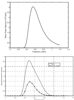
where β is the wave incidence angle related to the ship. The high frequency motion of the ship is then obtained by the time realization of the power spectrum function Pii. Figure 3 illustrates a typical
wave spectrum, for a 5.0m significant wave height and 11s peak period, considering the Pierson-Moskowitz description of irregular sea. Power spectra of sway motions are also presented, considering both the barge and the shuttle tanker. It should be emphasized that the peak frequency of motion spectrum may not be the same as that of the wave, due to the shape of RAO function, as can be seen in Fig.4.
0 0.2 0.4 0.6 0.8 1 1.2 1.4 1.6 1.8 2
0 0.1 0.2 0.3 0.4 0.5 0.6 0.7 0.8 0.9 1
Frequency (rad/s)
R
A
O
s
w
a
y
Shuttle tanker Barge
Figure 3. Sway RAO for a tanker and a barge under beam sea wave incidence.
0 0.2 0.4 0.6 0.8 1 1.2 1.4
0 0.5 1 1.5 2 2.5 3 3.5 4 4.5
Frequency (rad/s)
W
a
v
e
P
o
w
e
r
S
p
e
c
tr
u
m
(
m
2/r
a
d
/s
)
0 0.5 1 1.5 2 2.5 3 3.5 4
0 0.2 0.4 0.6 0.8 1 1.2 1.4
Frequency (rad/s)
S
w
a
y
p
o
w
e
r
s
p
e
ct
ru
m
(
m
2
/r
a
d
/s
)
Barge Shuttle Tanker
Figure 4. (Up) Wave power spectrum (5.0m wave height and 11s peak period). (Down) Spectrum of sway motion for a tanker and a barge under beam sea wave incidence.
Kalman Filter Design
Such models consider linearization about small heading angles, linear damping approximation, linear wave response, and others simplifications.
Being X and Y the position of the central point of the vessel (assumed to be coincident with the vessel center of mass), ψ the heading angle and disregarding non-linear terms, the low frequency motion can be described by:
)
(T E
1 3x3 L 1 3x3 L 3x3 3x3 3x3 3x3
L F F
M 0 ω M 0 x C 0 I 0
x +
+ + − = − − ɺ (3)
wherexL=
(
XL YL ψL XɺL YɺL ψɺL)
T, FT are thrusters forces andmoment vector, FE are low frequency environmental forces and
moment vector, M is the mass matrix of vessel and C is a damping matrix. The subscript L is related to low frequency motion. In this model, it is assumed that the heading angle is less than 20o, approximately, during the motion. ω L
is a 3x1 vector containing zero-mean Gaussian white noises processes with covariance matrix QL ( L~ (0,QL)
ω
N ).
The forces FE are slowly varying unknown variables, and can be
modeled by:
FL E
ω
F
ɺ
=
(4)Where ωωωωFL is a 3x1 vector containing zero-mean Gaussian white
noises processes with covariance matrix QFL (ωωωωFL ~N(0,QFL)). Finally, high frequency motions can be modeled by (Balchen et al., 1980): H H H ω I 0 x I I I 0 x 3x3 3x3 3x3 3x3 3x3 3x3 + − − = 0 2
0 2ζω
ω
ɺ (5)
where
(
)
TH H H H H H
H= ∫X dt ∫Y dt ∫ψ dt X Y ψ
x , ω H
is a 3x1 vector containing zero-mean Gaussian white noises processes ( H ~N(0,QH)
ω
) and H represents high frequency. The parameter ζ is the relative damping ratio of the motions, and was set as 0.1. The parameter ω0 should be the peak frequency of the motion power spectrum, which is close to the peak frequency of the wave spectrum, as explained in the previous section.
The measured signals z are given by:
+ + + + + + = ψ ψ ψ v v Y Y v X X H L Y H L X H L z (6)
where v is a 3x1 vector containing zero-mean, Gaussian white noise processes (v~N(0,R)).
Equations (3), (4), (5) and (6) were written as a discrete-time state space model and applied to a standard Kalman Filter. For the sake of simplicity, the matrixes QL, QH , QFL and R are considered
diagonal in real applications.
It should be emphasized that the Kalman Filter estimates the components xH and xL and also low frequency environmental forces
FE.
From now on, only one degree of freedom will be considered. Such simplification disregards the coupling between sway and yaw, presented in Eq. (1). Being x the controlled motion (surge, sway or
yaw), and x the vector containing all Kalman filter model variables
x =
(
xL,xɺL,∫
xHdt,xH,FE)
T , the previous equations transform as:ω
. .
.x B E
A
xɺ= + FT+ (7)
v
z=H.x+ (8)
− − − = 0 0 0 0 0 0 2 0 0 0 1 0 0 0 / 1 0 0 / 0 0 0 0 1 0 0 2 0 ζω ω m m c A ; = 0 0 0 / 1 0 m B ; = 1 0 0 0 1 0 0 0 0 0 0 / 1 0 0 0 m
E ;
(
1 0 0 1 0)
= H ; = FL H L ω ω ω ω
Where m is the total mass related to the controlled motion (considering the added mass) and c is the damping term presented in matrix C of Eq. (3).
The following discrete version of Eq. (7) is used in the Kalman filter algorithm, being ∆t the sampling time:
t t t k v k k z k k F k k T ∆ = ∆ = + ∆ = + = − + − + − = . ; . ; . ] [ ] [ ] [ ] 1 [ . ] 1 [ . ] 1 [ . ] [ E Γ B ✝ I A Φ H.x ω Γ ✝ x Φ x (9)
Being x the a priori estimate and xˆ the a posterior estimate of state vetor, X the error matrix covariance and K the Kalman gain matrix, the discrete Kalman filter is given by (Cadet, 2003):
Prediction T T T k k k F k k Γ Q Γ Φ X Φ X ☛ x Φ x . . ]. [ ˆ . ] 1 [ ] [ . ] [ ˆ . ] 1 [ + = + + = + Correction
(
)
(
)
(
[ ].)
. [ ] ] [ ˆ ] [ . ] [ ]. [ ] [ ] [ ˆ ]. [ . . ]. [ ] [ 1 k k I k k k z k k k k kk T T
X H K X x H K x x R H X H H X K − = − + = + = − (10) with = FL H L x Q Q Q 0 0 0 0 0 0 Q33
The frequency ω0 must be estimated, since it plays an important role in the filter performance. Commercial DPS contains algorithms to perform such on-line estimation, but the complete mathematical formulation is not given away by the manufacturers. Ljung (1987) presents several methods that can be applied in this problem, and in the present work the Recursive Prediction Error Method was adopted. The same method was used in the seminal work of Balchen et al. (1976).
− + − − − = − + − + − = 2 2 2 2 0 0 ] [ ]. 1 [ ] [ . ] 1 [ ] 1 [ . 1 ] [ ] [ . ] [ ]. 1 [ ] [ ]. 1 [ ] 1 [ ˆ ] [ ˆ k k P k k P k P k P k k k P k k P k k ψ λ ψ λ ε ψ λ ψ ω ω (11)
where λ is the forgetting factor (taken as 0.996 in the present work),
0 ˆ ]
[ =−∂
ε
∂ω
Ψk , P[k] is an estimate of cov(Ψ[k]). The sensitivity function Ψ[k] can be evaluated by:
0 0 0 ˆ ] [ ˆ ]) [ . ] [ ( ˆ ] [
ω
ω
ω
ε
∂ ∂ ≅ ∂ − ∂ − = ∂ ∂ − =Ψk zk Hxk H xk (12)
Using Eq.(10), one can show that
] [ ]. [ . ˆ ] [ . ] [ . ˆ ] 1
[k k FT k Kk εk
Φ
✁
x
Φ
x + = + + , being ˆ (ωˆo)
Φ Φ = , leading to:
(
)
.[ ] ˆ ] [ . ˆ ] [ ]. [ ] [ . ˆ ˆ ˆ ] [ ]. [ . ˆ ˆ ] [ . ˆ ˆ ] 1 [ 0 0 0 0 0 k k k k k k k k kε
ω
ε
ω
ω
ε
ω
ω
∂ ∂ + + ∂ ∂ + + ∂ ∂ + ∂ ∂ = ∂ + ∂ K Φ K x Φ K Φ x Φ x (13)disregarding the dependency of K[k] on ωˆ0[k], Eq. (13) and (12) lead to the following algorithm to evaluate the sensitivity function:
[
]
0 0 0 0 ˆ ] 1 [ ] 1 [ ] [ ˆ . ˆ ˆ ˆ ] [ . ]. [ . ˆ ˆ ] 1 [ω
ω
ω
ω
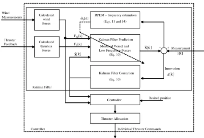
∂ + ∂ = + Ψ ∂ ∂ + ∂ ∂ − = ∂ + ∂ k k k k k I k x H x Φ x H K Φ x (14)Figure 5 presents a block diagram of the Kalman filter and the controller, which will be analyzed in the next section. It must be noticed that DP systems normally contain a feed forward loop to compensate for wind effects. Wind speed and direction are measured by anemometers, and the forces are worked out using the wind coefficients of the ship. Such forces are directly compensated by the controller, and they are counteracted before causing a positioning error. These estimates are also used by the Kalman filter, which must subtract them from the total thrust forces, resulting the parcel of thrust responsible for current and wave compensation. In the present work, such feed forward loop is not considered.
Model of Vessel and Low Frequency Forces
(Eq. 10) Kalman Filter Prediction
] [k x Measurement z[k] + _ (Eq. 10) Kalman Filter Correction
Innovation
]
[k
ε Thruster
Feedback Calculatedthrusters
forces
FT[k]
] [
ˆk
x
(Eqs. 11 and 14) RPEM – frequency estimation ]
[
ˆ0k
ω Wind
Measurements Calculatedwind
forces
Controller FW[k]
Desired position
Thruster Allocation
Individual Thruster Commands Kalman Filter
Controller
Figure 5. Kalman filter and controller block diagram.
Model-Reference Adaptive Controller Design
The idea behind the so-called model-reference adaptive control is to design a controller whose action on the plant under study is such that its response tracks that of a pre-established dynamic system, which is otherwise known as the reference model. Hence the name model-reference adaptive control (MRAC for short). The dynamic behavior of the reference model is represented by Eq.(15) and the plant dynamics is given in Eq.(16). A complete derivation of the MRAC can be found in Slotine and Li (1991).
) t ( u y k y c y
mMɺɺM+ MɺM + M M = c (15)
) t ( u y c y
mɺɺ+ ɺ= (16)
Note that for the present offshore operation, K=0, which basically means that the vessel is deprived of any sort of mooring lines whatsoever. We shall now introduce z(t):
z(t)=yɺɺM−β −1eɺ β0e (17)
where e=y−yM, β0 and β1 are positive constants such that
0 1 2+β +β
s
s is a stable (Hurwitz) polynomial . It follows from this definition that e is expected to converge asymptotically to zero (the plant matches the reference model). Now, let us define the
vector v = T
y t
z() ]
[ ɺ and the vector of estimated parameters â(t)
= T
a aˆ ˆ ]
[ 2 1 . In doing so, we have laid the basis to define the control
law, which is given by:
y a t z a t
u()=ˆ2 ()+ˆ1ɺ (18)
At this point, all that is left is to evaluate the law for the adaptation mechanism. The error (e=y−yM) dynamics can be written as: ) ( ~ ). ( 1 2 0
1e e a t t
e T
a v = +
+
β
ɺβ
ɺ
ɺ (19)
where ã(t)=â(t)-a(t). Equation (19) can be rewritten in the state-space form as:
+
= v a~
a b Ax x T 2 1 ɺ
with A =
−
− 0 1
1 0
β
β ; b =
1 0
; x = e e ɺ (20)
Introducing the matrices ΓΓΓΓ , G and QC, being ΓΓΓΓ and G
symmetric positive definite constant matrices, T C
Q G A
GA+ =− ,
0
>
= T
C C Q
Q , for a chosen QC. The adaptation law is then given
by:
(
)
Γ vb G.xT . . . 1
2 =−
T aˆ a
ˆɺ ɺ (21)
Figure 6. Model-reference adaptive controller
Convergence properties can be proved using the following Lyapunov function and its time derivative:
ã
Γ
ã Gx x ã)
V(x, = T + T −1
x Q x ã
Γ
2ã Gx vb 2ã x Q x
V C
T 1 T T T T
− = +
+ −
= −ɺ
ɺ
C (22)
It is possible to show the convergence of x using Barbalat´s lemma. Therefore with the adaptive controller defined by both the adaptation and the control law, x converges to zero. The condition for parameter convergence can be shown to be the persistent excitation of the vector v.
By using β0 = kM/mM and β1 = cM/mM, it goes without saying that
the polynomial 1 0
2+β +β
s
s will be stable. Substituting Eq.(18) in Eq.(16), one obtains the following closed loop dynamics:
y aˆ ) t ( z aˆ y c y
mɺɺ+ ɺ= 2 + 1ɺ (23)
Using Eq. (17) and (15), Eq.(23) can be written as:
y aˆ ) y y m
) t ( u ( a ˆ y c y m
M
c ɺ ɺ
ɺ ɺ
ɺ+ = 2 −β1 −β0 + 1
(
c aˆ aˆ)
y aˆ y u(t) aˆ m . y a ˆ m . m
c M
M + + − + =
0 2 1 1 2 2 2
β
β ɺ
ɺ
ɺ (24)
Since the tracking error converge to zero, Eq.(24) converges to the reference model Eq.(15), what is only possible if aˆ2→m and
c aˆ1→ .
The analogy between a PD controller and the previously derived MRAC is obtained by means of Eq. (18), that can also be written as:
M y a ˆ e a ˆ y aˆ e a ˆ ) t (
u =− 2β1ɺ+ 1ɺ− 2β0 + 2ɺɺ
where the first and second terms are responsible for the derivative action and the third term gives the proportional action. For the surge motion, in which the damping factor c is extremely small (c<<cm),
the equivalent constant Pr and D gains are given by:
M M R
m k . m aˆ
P =− 2β0=− ;
M M m c . m aˆ
D=− 2β1=− (25)
Case study
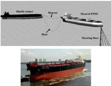
The controller was implemented in a numerical simulator, considering a real shuttle vessel operating in Brazilian waters during an offloading operation (Fig. 7). The main properties of the tanker in both, ballasted and loaded, conditions are presented in Table 1.
Moored FPSO
Mooring lines Hawser
Hose Shuttle tanker
Figure 7. (Up) Offloading operation; (Down) Picture of shuttle tanker in ballasted condition.
Table 1. Tanker main properties.
Property Full load condition Ballasted condition
Length (L) 260 m
Beam (B) 44.5 m
Draft (T) 16.1 m 6. 4 m
Mass (M) 156,310 ton 58,783 ton
Surge Added Mass (M11)* 1,560 ton 8,510 ton * Low frequency
A 12h offloading operation was simulated, throughout which the tanks of the ballasted ship are loaded up with oil getting transferred in from the FPSO. The shuttle tanker is kept aligned with the FPSO, at a distance of approximately 100m. Therefore, surge motion control is critical, due to the risk of collision as well as hose rupture. So, FPSO position must be monitored and, in case of large amplitude motions, DPS must relocate the shuttle in order to keep a safe distance from the FPSO. In order to analyze controller performance, it was considered corrections of 20m every 30min. This simulation tries to recover the real control approach used in DPS installed in shuttle vessels. In order to save fuel, the shuttle tanker does not follow all motions of FPSO, being only relocated when the FPSO presents a large displacement (Bravin and Tannuri, 2004). Figure 8 shows the environmental condition and the set-point considered in the simulations.
Shuttle Tanker
FPSO 1 hour
20m
Surge set-point
1,0m/s Current
2,0m height,10s period Wave
Figure 8. Surge set-point and environmental conditions acting upon the shuttle tanker.
× ×
=
10 10
3 3
10 2 . 1 0 0
0 6 . 2 0
0 0 10 4
x
Q ;R = 1 ;
× ×
= 10 6
1 2
10 8 0
0 10 4 x
Γ ;
6 10 5 . 6 1 0
0
1 −
× ×
=
2x1 C
Q
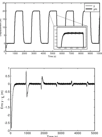
Figure 9 shows the simulation result considering the adaptive control. The reference model is a second order system with a natural period of 200s and damping factor of 1.0 (no overshoot). The reference model is tracked with good accuracy by the ship, despite the mass variation, with no performance loss. After a short transient, the tracking error e = y-ym is reduced to values smaller than 0.5m,
being mainly represented by the non-controlled high-frequency motions. Figure 10 presents control force, which gets higher during the simulation, due to an increase in the mass, damping, wave and current forces.
The adaptive controller estimation of the components of vector â(t) (mass and damping, as already explained), are shown in Fig. 11. The mass estimation presents very good accuracy and an oscillatory behavior was found in damping estimation. This fact was expected, since damping effect in surge motion is extremely small, what is confirmed by the very good performance of the system (Fig. 9) despite such estimation error. Figure 12 confirms that Kalman filter high frequency motion estimation works properly. The estimation of the surge motion peak period converges to 12.5s, recovering the value theoretically evaluated by Eq.(2). As already mentioned, this value is close to the peak period of waves (10s in the present case).
0 1000 2000 3000 4000 5000 6000 7000 8000 9000 10000
-5 0 5 10 15 20 25
Time (s)
D
is
p
la
c
e
m
e
n
t
(m
)
x xm
4600 4800 5000 5200 5400
19.2 19.4 19.6 19.8 20 20.2
y ym y ym
0 1000 2000 3000 4000 5000
-3 -2.5 -2 -1.5 -1 -0.5 0 0.5 1
Time (s)
E
rr
o
y
ym
(
m
)
Figure 9. (Up) Actual Surge position (y) and reference-model output (ym)
(Down) Tracking error e=y−ym.
0 0.2 0.4 0.6 0.8 1 1.2 1.4 1.6 1.8 2
x 104 -2.5
-2 -1.5 -1 -0.5 0 0.5 1 1.5 2 2.5x 10
6
Time (s)
C
o
n
tr
o
l
F
o
rc
e
(
N
)
Figure 10. Control force delivered to vessel thrusters.
0 0.2 0.4 0.6 0.8 1 1.2 1.4 1.6 1.8 2
x 104
4 5 6 7 8 9 10 11 12x 10
7
Time (s)
M
a
s
s
(
k
g
)
Estimated Mass Actual Mass
0 0.2 0.4 0.6 0.8 1 1.2 1.4 1.6 1.8 2
x 104 1.5
2 2.5 3 3.5 4 4.5
5x 10
4
Time (s)
D
a
m
p
in
g
C
o
e
f.
(
N
/m
/s
)
Actual Damping Estimated Damping
Figure 11. Parameter estimation. (Up) Mass ; (Down ) Damping.
1. 17 1 .1 75 1. 18 1 .1 85 1.1 9
x 1 04
-0.1 -0 .05 0 0 .05 0.1 0 .15
H igh freq ue n c y m ot io n (m )
A c t ua l M o tio n E s t im at ed M o tio n
0 0. 2 0 .4 0. 6 0 .8 1 1.2 1. 4 1 .6 1. 8 2
x 1 04
4 6 8 10 12 14 16
2π / ω0 e s tim a tio n (s )
Tim e (s )
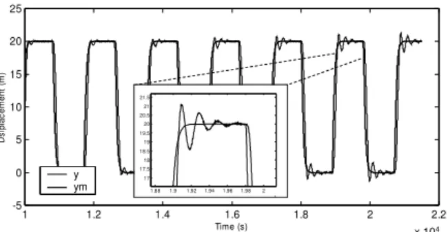
The fixed-gain PD controller was also applied to the problem, and the simulation output is displayed in Fig. 13. The performance loss during the offloading operation becomes evident as the mass and other dynamic properties of the ship changes. Since the P and D gains associated with the controller was evaluated by Eq. (25) considering the ballasted mass of the ship, the performance of the controller is better in the beginning of the operation, getting progressively worse as the ship’s inertia increases. As a result, the overshoot in the closed-loop response increases, which may cause dangerous approximations of the ships.
1 1.2 1.4 1.6 1.8 2 2.2 x 10⁴ -5
0 5 10 15 20 25
Time (s)
D
s
ip
la
c
e
m
e
n
t
(m
)
y
ym 1.88 1.9 1.92 1.94 1.96 1.98 2
4
17 17.5 18 18.5 19 19.5 20 20.5 21 21.5
x 104
Figure 13. Actual position (y) and set-point (ym) (Shuttle tanker).
A simple analysis shows that a constant-gain controller may lead to oscillatory behavior as the mass increases. In fact, the following equation represents the closed-loop transfer function of surge motion:
R R
P s ) c D ( ms
P Ds
+ + +
+
2 (26)
The closed loop equivalent damping factor (ζ) and natural frequency (ωn) are then by:
m PR n =
ω ;
m . P
c D
R 2
+ =
ζ (27)
As expected, for an increasing mass, the damping factor decreases, and the closed loop system may become equivalent to a sub-critically damped oscillator. Furthermore, the natural frequency of the oscillator also decreases.
Conclusions
This work presented the application of the model-reference adaptive control technique to DPS’s cascaded with the commonly used adaptive Kalman filter. The controller was applied to a dynamic-positioned shuttle tanker exposed to environmental forces issuing from the interaction of waves and currents with the floating vessel, over the course of an offloading operation. The results showed that a good performance can be assured throughout the operation, despite the significant variations in dynamic properties
undergone by the vessel thanks to oil transfer. The adaptive algorithm was able to estimate the mass of the vessel with a good accuracy – provided a persistent excitation is fed into the system – as well as to properly tune the controller gains. For the sake of comparison, a fixed-gain PD controller was tested out in the very same situation, and it was shown that such controller fails to cope with substantial changes imparted to the vessel dynamic properties, leading to a loss in performance as the operation unfolds.
Acknowledgements
This work has been supported by Petrobras and the State of São Paulo Research Foundation (FAPESP – Processes no. 02/07946-2 and 03/12330-3). A CNPq research grant, process no.302450/2002-5, is also acknowledged.
References
Aarset, M.F., Strand, J.P. and Fossen, T.I., 1998, “Nonlinear Vectorial Observer Backstepping With Integral Action and Wave Filtering for Ships”,
Proceedings of the IFAC Conference on Control Applications in Marine Systems (CAMS'98), Fukuoka, Japan, pp.83-89.
Balchen, J.G., Jenssen, N.A. and Saelid, S., 1976, “Dynamic Positioning using Kalman Filtering and Optimal Control Theory”, Proceedings of IFAC/IFIP Symposium on Automation in Offshore Oil Field Operation, Bergen.
Balchen, J.G. et al., 1980, “A dynamic positioning system based on Kalman filtering and optimal control”, Modeling, Identification and Control, Vol. 1, No. 3, pp. 135-163.
Bravin, T.T. and Tannuri, E.A., 2004, “Dynamic Positioning Systems Applied to Offloading Operations”, International Journal of Maritime Engineering (IJME), Vol 146 (2004), Part A2.
Bray, D., 1998, “Dynamic Positioning”, The Oilfield Seamanship Series, Volume 9, Oilfield Publications Ltd. (OPL).
Cadet, O., 2003, “Introduction to Kalman Filter and its use in Dynamic Positioning Systems”, Proceedings of Dynamic Positioning Conference, September 16-17, Houston, USA.
Fossen, T.I., 1994, “Guidance and Control of Ocean Vehicles”, John Wiley & Sons, 479p.
Katebi, M.R., Grimble, M.J. and Zhang, Y. (1997), “H∞ robust control design for dynamic ship positioning”, IEE Proc. Control Theory Appl, Vol.144, No.2, pp. 110-120.
Kongsberg Simrad, 1999, “Operator Manual Kongsberg Simrad SDP (OS)”, Rel 2.5, Norway, 412 p.
Ljung, L., 1987, System Identification, Theory for the User, Prentice Hall, Inc., Englewood Cliffs, New Jersey.
Saelid, S., Jenssen, N.A. and Balchen, J.G., 1983, “Design and Analysis of a Dynamic Positioning System Based on Kalman Filtering and Optimal Control”, IEEE Transactions on Automatic Control, Vol.AC-28, No.3, pp. 331-339.
Slotine, J.J.E.; Li, W. , 1991, “Applied Nonlinear Control”, Prentice Hall, New Jersey.
Tannuri, E.A., Donha, D.C. and Pesce, C.P., 2001, “Dynamic Positioning of a Turret Moored FPSO Using Sliding Mode Control”,
International Journal of Robust and Nonlinear Control, Vol.11, pp.1239-1256, May.