Elastoplastic finite element analysis for wet multidisc brake during lasting braking

ELASTOPLASTIC FINITE ELEMENT ANALYSIS FOR WET MULTIDISC

BRAKE DURING LASTING BRAKING

by

Zhanling JIa,b, Yunhua LI*a,b, Sujun DONG*c, Peng ZHANGa, and Yunze LIc

a_{School of Automation Science and Electrical Enginering, Beihang University, Beijing, China} b_{School of Mechanical Enginering, North China University of Water Resources and Electric Power,}

Zhengzhou, China

c_{School of Aeronautic Science and Engineering, Beihang University, Beijing, China}

Original scientific paper DOI: 10.2298/TSCI141121016J

Addressed to serious heat degradation problem of the braking continuously per-formed in the drag brake application for a long time, finite element analysis for bidirectional thermal-structure coupling is adopted to investigate temperature and stress when material properties are temperature-dependent. Based on the constitu-tive relations of heat transfer and strain-stress, 3-D transient finite element equilib-rium equations with many kinds of boundary conditions for bidirectional ther-mal-structure coupling were derived. It was originally presented that start time, location, severity, and evolution laws of plastic deformation were depicted using dimensionless stress distribution contour with the yield limit related to tempera-ture. The change laws of plastic element number and contact area vs. braking time were expressed by plasticity ratio and contact ratio curves, respectively. The laws revealed by the numerical calculation results are in accordance with the objective perception and reasoning.

Key words: wet multidisc brake, elastic-plastic analysis, lasting braking bidirectional thermal-structure coupling

Introduction

The brake is a crucial component of the vehicle, the construction machinery, the ma-nipulative steering engine and the brake system of an aircraft. The wet brake is widely used in the large-scale machineries and the special operating environment due to its low wear and easily increased brake torque features. When the vehicle is running at emergency braking, repeated braking or uniform velocity on a long sharp downhill, the braking is performed rapidly, fre-quently or lastingly for a long time. At the time a large amount of kinetic energy and potential energy will be transformed into heat, if the heat cannot be released to the surroundings timely because of the cooling restriction, heat accumulation and temperature rise will occur. When temperature rises to a certain extent, braking performance degradation is severe on account of mechanical, physical, and chemical factors, thus the vehicle accidents for braking problem are frequent, even fatal traffic accidents are caused to endanger driving safety. The heat problems

generated by friction also exist in engagement operation of the steering engine brake and master clutch between main hydraulic pump and the aircraft engine. At present, thermal analysis and thermal control researches on the brake and clutch have become a very attracting issue.

Many researches related to the brake have been carried out from different aspects, such as temperature [1-3], plasticity [4-6], thermo-elasticity [7-13], thermo-plasticity [14-18]. By the analysis for previous research information, it is summarized that the key problems exist as fol-lows. They mainly focus on the temperature field and thermo-elasticity analysis of the brake or clutch. Since Biot [19] developed the coupled theory of thermo-elasticity in 1956, thermo-elas-tic coupling has been continually extended to generalization and depth. However, numerical so-lution method mainly adopts the sequential coupling, which mainly considers that temperature field influences stress field, and ignores that stress field influences temperature field, even tem-perature influences material properties, consequently it is difficult to systematically research on thermo-elasticity. Thermo-plasticity researches are primarily addressed to residual stress, how-ever researches on plasticity evolution lawsvs.space and time are less during loading.

In addition, there has been no better means and ways in plasticity visualization de-scription when the yield limit relates to temperature. Elastic-plastic behavior was represented through the yield surface and the stress path [20]. The plastic state was judged according to non-linearity of the strain-stress curves [21]. The plastic regions were demonstrated by sche-matic diagram [22], but the problems were 2-D and referred not to thermal physics. Plasticity was decided in the light of the comparison of the time-stress curve with the time-yield limit curve [23]. However the deformation only at some locations was evaluated. The plastic regions were confirmed by combining with temperature field and stress field [24], but it could not accu-rately display elastic-plastic regions.

It is a goal of thermal analysis and thermal control to recognize and solve a series of problems induced by temperature rise during frictional braking process. For this purpose, tem-perature, stress and plastic deformation of wet multidisc brake are investigated by bidirectional thermal-structure coupling in the paper.

Problem formulation

For heat control of wet clutches and brakes, the analysis of heat problems induced by their engagement and structure deformation induced by heat must be conducted. Taking the brake used in the heavy vehicle running in the sharply inclined long tunnel for example here, heat fading problem of the brake is studied by thermal analysis for friction lining and elas-tic-plastic analysis for steel disk.

In order to keep the vehicle uniform and stable under gravity component downhill, the brake is continuously engaged for a long time. There will be a lot of potential energy trans-formed into heat energy at the time. For the vehicle driving in a mining tunnel, heat dissipation is more inconvenient, temperature rising speed of the brake is faster.

Figure 1 is the inner structure of the brake and boundary conditions and load of a fric-tion pair. Steel disks are connected to the static components by inner gears. Core disks are con-nected to the dynamic components by outer gears. Friction linings are fixed at the two sides of core disks. The radial and circumferential grooves are processed on friction linings, which play an important role in cooling and taking wear debris. When pressure oil is released from chamber 1 and chamber 2, parking brake is remained by a disc spring. When pressure oil is released from chamber 1 and filled to chamber 2, the brake is released. When pressure oil is filled to chamber 1 and chamber 2, dynamic brake is performed.

Mathematical models for bidirectional thermal-structure coupling

Heat transfer model

Material properties are supposed as linear piecewise interpolation functions of tem-perature. Heat conduction equation for isotropic material and bidirectional thermal-structure coupling is [19]:

rc T T b

t T e

t x k T T

x y k T T

y

( )¶ ( ) ( )

¶

¶ ¶

¶ ¶

¶ ¶

¶ ¶

¶ ¶

+ = é

ëê

ù ûú+

é ë ê

0

ù û ú + é

ëê

ù ûú+ ¶

¶

¶ ¶ z k T

T z q

( ) _v (1)

whereT₀b(¶e/¶t) is an additional term induced by deformation energy, andq_vis the internal heat generation rate.

There are two kinds of boundary conditions in eq. (1): temperature boundary condition S₁and heat flow density boundary conditionS₂. The brake has onlyS₂, and the solution area is W. The external heat flux onS₂includes the heat flow densities generated by the friction contact, convection, and radiation, and they are denoted byq,h(T–T_f), andes(T4_–T

e4) separately. Con-tinuity conditions at the sliding interface are p> 0,T_I=T_II,q=q_I+q_II=f(p,v,t,T)wp(t)r, and p= 0,T_I¹T_II,q_I=q_II= 0. Initial condition isT|_t=0=T₀.

Figure 1. The inner structure of the brake and detail view of a friction pair subjected to thermal and mechanical load

Boundary conditions can be transformed:

-k T - - = + - +

-x n k T

yn k T

zn q h T T T T x y

x y z e

¶ ¶

¶ ¶

¶

¶ ( f) es( ) ( , ,

4 4 _z)Î_S

2 (2)

wheren_x,n_y, andn_zare cosine value of the included angle between the outward normal direction of the boundary and x-, y-, and z-axis, respectively.

The last item at the right end in eq. (2) is rewritten:

es(T4 -T_e4)= ¢k T( -T )

e (3)

wherek¢ =es(T2 +T_e2)(T +T ) e .

The research region is discretized as many little elements, temperature distribution function in each element is:

T x y z t N x y z T t_{i i} N T e i

m

( , , , )=å ( , , ) ( )=[ ]{ }

=1

(4)

Galerkin method is applied to each element, and eq. (1) is rewritten:

N

x k T T

x y k T T

y z k T T z i ¶ ¶ ¶ ¶ ¶ ¶ ¶ ¶ ¶ ¶ ¶ ¶ ( ) ( ) ( ) é ëê ù ûú+ é ë ê ù û ú + é

ëê ù ûú+ ì í î ü ý þ

-- é +

ëê

ù ûú

ò

N T c T T t T e t V v i d d W

r( ) ( )¶ b

¶ ¶ ¶ 0 =

ò

The first three items in eq. (5) are integrated by parts, respectively, which are rewrit-ten:

N

x k T T

x V k T

T

x N n S k T T

i i x

¶ ¶ ¶ ¶ ¶ ¶ ¶ ¶ ( ) ( ) ( ) é ëê ù ûú ì í î ü ý

þd = d - x

N x V i S ¶ ¶ d W W

ò

ò

ò

y k T T

y V k T

T

y N n S k T T

i i y

¶ ¶ ¶ ¶ ¶ ¶ ¶ ¶ ( ) ( ) ( ) é ë ê ù û ú ì í î ü ý þ = -d d y N y V i S ¶ ¶ d W W

ò

ò

ò

z k T T

z V k T

T

z N n S k T T

i i z

¶ ¶ ¶ ¶ ¶ ¶ ¶ ¶ ( ) ( ) ( ) é ëê ù ûú ì í î ü ý

þd = d - z

N z V i S ¶ ¶ d W W

ò

ò

ò

Substituting eqs.(4), (6), (7), and (8) into eq. (5) yields thermal equilibrium equation of every element of transient heat transfer problem, which includes all kinds of boundary condi-tions for bidirectional thermal-structure coupling in the matrix form:

([k ] [k ]){ }T ([ ] [ ] )c c { }T { } { } [

t Q Q Q

e e e e

t h e v q t

d

d e

+ + + = - + ] (9)

where

[ ]c c T( )[N] [N] V; [ ]c T T u x T v y T

= = æ

è ç ö

ø ÷ + æ

è

r d _{e 0}b ¶

¶ ¶ ¶ ¶ ¶ ¶ ¶ çç ö ø

÷÷ + æ_èç ö ø ÷ é ë ê ù û ú ò ò = ¶ ¶ ¶ ¶ ¶ T w

z N N V

k k T

T [ ] [ ] ; ] ( ) d [ _t W W [ ] [ ] [ ] , [ ] ( N x N x N y y N z N

V k h

T T T

¶ ¶ ¶ ¶ ¶ ¶ ¶ ¶ ¶ ¶ ¶ + + æ è çç ö ø

÷÷d _h = ò + ¢ ò

= = + ¢

k N N S

Q N q V Q hT k T N

T S e T f )[ ] ; } [ ] , [ ] ( )[ d

{ _{v v}d _{t e}

e

2

W

]T , { }e [ ]T S S

S Q N q S

d _q = ò d

ò ò

2 2

W

[ ( )]{C T T&} [ ( )]{ } { ( , )}+ K T T = Q T t (10) where

[ ( )]K T = ([k_t]+[k_h] ), [ ( )]C T = ([ ] [ ] ), { ( , )}c + c_e Q T t = ({Q_v}e { }e [ ]) e n e n e n Q Q e e e - + å å å = =

= q te

1 1

1

Equation (10) is re-written in time difference form:

[ ]

[ ] { } ( ){ ( , )} { ( , )

C

t K T Q T t t Q T t t

D + æ è ç ö ø ÷ = - - +

-q _t 1 q 2D q D _}+æ[ ]-₍ - _{)[ ] { }}

è

ç ö

ø ÷ -C

t K T t t

D 1 q D(11)

whereqis the Euler parameter,qÎ[0, 1], hereq= 2/3.

Thermo-elastic-plastic model

Due to temperature-dependent physical properties and plasticity, loading mode by step is used. When each load step is smaller, strain increment-stress increment in the plastic re-gion can be written:

D_{{ } [ ] ( { }s} = _D D _e -D_{{~} )e} +D_{~}s

ep T T (12)

where D_{{~}e { }a} [ ] _{{ }s} { }a _{{ } ,} D_{~}s

T T

D

T T T T T

=æ + +

-è ç ö ø ÷ -d d d d 1

0 D =

¢ +ìí î ü ý þ [ ] { } { } [ ] { } D H T T

H_T D

T ¶ ¶ ¶ ¶ D ¶ ¶ ¶ ¶ s s s s s s Supposing that a body is imposed by volume force {p} = {p_x,p_y,p_z}T_{, surface force} { }p = {p_x,p_y,p_z}T_{, and concentrated force {P} = {P}

x,Py,Pz}T, all the amounts are changed by linearization during small incremental time dt. In the light of the incremental virtual work prin-ciple, the following equation is formed:

[ds d e_x (d _x)+ds d e_y (d _y) +ds d e_z (d _z) +dt d g_xy (d _xy)+dt d_yz (dg t d g

d d d

yz zx zx

v

x y z

v

p u p p w

) ( )]

( ) ( ) ( )

+

-ò

- + +

d d d

[d d d dv d d ] [ ( ) ( ) ( )]

[ ( )

d d d d d d d d

d d

v p u p v p w s

P u

x y z

S v

x

- _ò + +

-ò

-d d d

d

s

+dP_yd(dv)+dP_zd(dw)] 0= (13) The research region is discretized as finite elementse. Displacement {u} at any point in an element is expressed by nodal displacement {u}e_:

{ } [u = N]{ }u e ₍₁₄₎

The strain {e} is defined:

{ } [ ]{ }e = B u e ₍₁₅₎

Substituting eqs. (12), (14), and (15) into eq. (13) yields element stiffness equation in plastic regions is:

[ ]k e { }u e {F} { F} {F} { F} { }P

T e p e H e p e e

d = d + d - d + d + (16)

where

[ ]k e [ ] [ ] [ ], {B T D B F} [ ] [ ] ( {~} ) , {B D v F}

ep Te T ep T p

= d = d e d d e T

v v

H

e T

T ep T

N p v

F B d v F N

= ò ò = = [ ] { } , [ ] ( {~} ) , { } [ ] d d

{d } s d d { } , { }d dp v P e [N] {T dP}

S v = ò ò s

Results and discussion

Bidirectional coupling flow of temperature field and stress field

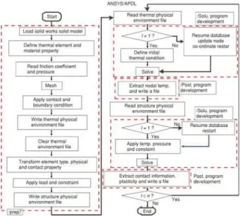
Figure 2 is the bidirectional ther-mal-structure coupling flowchart. The main technical points in the pro-cess are as follows. Multi-physics field is conveniently converted by physical environment file, data be-tween physical fields is transmitted by temperature results or data file. Owing to temperature-dependent physical properties and mutual effect of thermal and structure, loading by step and single frame restart are em-ployed.

Validation of numerical analysis method

One pole is fixed at the two ends, length l = 0.5 m, and diameterd = =i0.01 m, as shown in fig. 3. Its circumferential outer surface is heated by heat fluxq= 60000 W/m2_{, timet= 10 s, and} ini-tial temperatureT₀= 293 K. The pole is made of 45 steel, and its material properties are: r= 7850 kg/m3_{,c= 476 J/kgK,}

a= 11.59·10–6_{l/K, andE= 209·10}9_Pa.

Because of smaller radial size and higher thermal conductivity coefficient, tempera-ture of the heated pole basically keeps uniform everywhere and changes together, and lumped capacitance model can be adopted, thermal equilibrium equation is:

rcV T t qA d

d

= - (17)

Integrating the two ends of eq. (17) yields:

T qA

cV t C = - +

r 1 (18)

When heated timet= 0 s, the temperature can be expressed asT₀=C₁= 293 K. When heated timet= 10 s, the temperature can be expressed as:

T q l

c lt

10 ₂

025 293

60000 025 7850 476 001

= - + = -

-× × × p

p d

d

. r . . 10+293=35723. K

When heated timet= 10 s, the stress can be given as:

s₁₀ =a_{E T( 0} -_T50)=_{1159 10.} × -6×_{209 10 293}× 9₍ -_{35723. )}= -_{155.6 10}× 6_Pa

When the bidirectional thermal-structure coupling method is adopted and the pole is heated to 10 s, temperature and axial stress distribution contours are shown in figs. 4 and 5,

re-Figure 2. Bidirectional thermal-structure coupling flowchart

spectively. Temperature is from 355 to 359 K, axial stress is mostly from –170 to –150 MPa, what are consistent with the above calculation results after simplified conditions. Moreover, due to constant material properties and no plasticity considered, these results are completely same with that when the direct coupling method is used.

Analysis on the temperature field

When the brake is continuously engaged for 2300 s, temperature field distribution of multidisc friction pairs is shown in fig. 6. In the radial direction, temperature distribution ap-pears outer convex near the grooved regions, in contrast, that apap-pears inward concave at the non-grooved regions. The higher temperature regions at the inner and outer edges are in the shape of ellipses. From the profile, temperature at the two sides and the outer edge is lower due to more adequate heat dissipation, where temperature distribution shapes a parabolic type.

When the braking is performed at various time instants, temperature distribution of a friction lining is shown in fig.7. The conclusions are drawn from these figures are:

(1) Temperature is lowest at the interchange of the outer edge and radial grooves of the friction lining. Temperature at the outer edge is lower than that at the inner edge.

(2) Temperature difference rapidly becomes larger between the grooved regions and the non-grooved regions during short initial engagement time, cooling effect become more and more dramatic, so the relative high temperature area on the friction lining becomes smaller.

Figure 4. Temperature distribution contour of the pole, [K]

(for color image see journal web site)

Figure 5. Axial stress distribution contour of the pole, [Pa]

(for color image see journal web site)

Figure 6. Temperature field distribution of multidisc friction pairs att_{= 2300 s, [K]}

(3) Deformation at high temperature regions is larger, where contact status becomes worse and generated friction heat decreases, consequently as the braking time elapses, higher temperature regions continually move toward the inner edge, where hot spots and local burning loss easily occur.

(4) After a period of braking time, temperature rising speed becomes slow. After 1000 s, temperature basically remains unchangeable.

Temperature curves along the braking time at the selected locations of the friction lining are shown in fig. 8. These locations are located at MX, yellow region and MN in fig. 7(f), respec-tively. From the curves, it is seen that tempera-ture sharply rises at the initial engagement, after that temperature rising speed slows down. After 1000 s, due to friction coefficient decreasing and contact area reduced after deforming, gen-erated friction heat and heat conduction area be-come small, whereas cooling oil temperature rises more slowly, heat dissipation capability falls to a certain extent, it reaches a thermal equilibrium state.

Figure 7. Temperature field distribution of a friction lining at different braking time, [K] (for color image see journal web site)

Analysis on the structure field

When the brake is continuously engaged for 2300 s, stress and axial deformation dis-tribution contours of multidisc friction pairs are shown in figs. 9 and 10, respectively. The stress gradually gets higher from one side to the other, and the maximum is 743 MPa. Deformation is larger at the inner edge of the steel disks, which are acted together by friction heat, friction force and pressure, the maximum is 0.491mm.

The stress at a certain temperature to the yield limit at the temperature is defined as dimensionless stress, whose value indicates an element is in deformation state. If the value is less than 1.0, it represents extent of element deformation being close to plasticity. Otherwise it represents severity of an element in the plastic deformation. Dimensionless stress distribution contours of a steel disk are shown in fig.11 when the brake is in the drag brake application at var-ious time instants. In figs. 11 (b)-(f), the red regions indicate locations of plastic deformation, where the cracks easily produce. The analysis conclusions of fig. 11 are:

(1) The steel disk produces warping deformation, and plastic deformation occurs surrounding the inner edge earlier, as the braking time elapses, the regions of plastic deformation enlarge, after a certain time, which basically remain unchanged, but after material softening induced by temperature rise, deformation level decreases.

(2) At time 200 s, the maximum dimensionless stress is about 0.999, which is less than 1, what reveals stress of all the elements is less than the corresponding yield limit, and all the regions keep in perfectly elastic state and do not produce plastic deformation yet.

(3) At time 300 s, a small amount of elements nearby the inner edge produce plastic deformation, the maximum dimensionless stress is 1.003.

(4) At time 400 s, plastic deformation regions sharply enlarge with temperature rise, and deformation of the whole steel disk increases.

(5) At time 700 s, plastic deformation regions are larger, and the minimum dimensionless stress is over 0.95, what shows all elastic regions are close to plastic state, the regions where smaller dimensionless stress locates mainly concentrate around the circumferential and radial grooves.

Figure 9. Stress contour of multidisc friction pairs at braking timet_{= 2300 s [Pa]}

(for color image see journal web site)

Figure 10. Axial deformation contour of multidisc friction pairs at braking timet_{= 2300 s}

(6) During 700 s to 1100 s, deformation level gradually increases, but speed is very slow. (7) At time 2300s, compared with 1100 s, the regions where plastic deformation locates

basically remain unchanged. However, as temperature slightly rises, deformation level of the whole disk decreases.

The contact element number to the total element number on the contact interface is de-fined as contact ratio, time-contact ratio curve of a friction pair is shown in fig. 12. Figure 12(b) is the enlarged part of the interval shown in fig. 12(a). Temperature of friction linings and steel

Figure 11. Dimensionless stress contours of a steel disk at different braking time (for color image see journal web site)

disks sharply rises after short initial braking time, contact area between them rapidly de-clines, temperature continuously climbs with the braking time, but material softening is obvi-ous, deformation decreases, continuing for braking, temperature rising speed slows down, deformation slightly increases, especially plas-tic deformation can not recover, contact area decreases again, but whose speed slows, and contact ratio slowly falls. After a certain time, temperature increases in small amounts, mate-rial is further softened, elastic deformation slightly decreases, and contact ratio rises a bit again.

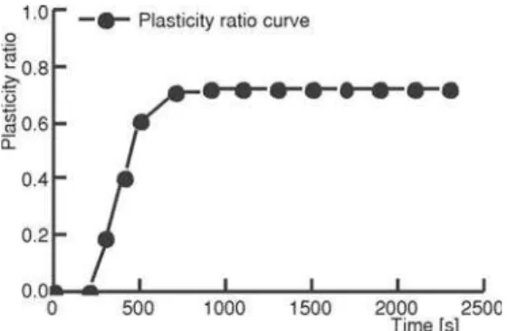
The plastic deformation element number to the total element number is defined as plasticity ratio. Time-plasticity ratio curve of a steel disk is shown in fig. 13. At the initial en-gagement phase, temperature is lower, deformation is in the elastic range, and plasticity ratio is 0. After 200 s temperature sharply rises, yield limit quickly falls, and plasticity ratio rapidly grows. After 700 s temperature more slowly increases or basically remains unchanged, plastic-ity ratio is approximatively a constant.

Discussions

There is no issue brought by lasting braking in the normal braking. Lasting braking co-mes from long down slope and large dropping-stroke winding system. At the moment, if the brake torque of the brake is used to balance the negative load and to suppress over-velocity, the serious injuries will be brought to the braking performances after lasting braking for 200 s. Prac-ticable methods to solve this problem can be considered from the two following aspects. One is forced lubricating and cooling to take enough frictional heat away, such as strengthening circu-lar flow of cooling oil, and spraying water or ventilating over the outermost housing. The other is to balance the negative load using the back-pressure and energy-recovery so as to decrease the brake moment, such as engine exhaust braking, balance valve, energy feedback recycling, and retarding pump.

Conclusions

The main conclusions are drawn by the above work as follows.

· As the braking time passes, temperature of multidisc friction pairs continually rises, but the speed becomes slow, especially during 700 s to 1000 s, after that temperature is roughly constant. Temperature is lowest at the interchange of the radial grooves and the outer edge on the friction lining, and the higher temperature regions continually move toward the inner edge.

· After braking time 200 s, plastic deformation produces in a small amount of elements at the inner edge. At braking time 1100 s, plastic deformation regions enlarge, and elastic regions are close to plastic state. Continuing for braking, plastic deformation regions basically remain unchanged, but deformation level of the whole disk decreases.

· By contact ratio curve, it can be concluded that contact area along the braking time declines then sharply increases during the initial engagement time 100 s, and slowly declines and increases again after that.

· By plasticity ratio curve, it can be concluded that plasticity ratio rapidly rises after 200 s, and number of plastic elements keeps invariable after 700 s.

The interaction of thermal and structure together under friction heat and mechanical load is better solved by bidirectional thermal-structure coupling method proposed in the paper. The spatial distribution laws and evolution laws with braking time of temperature and stress in an assembly unit and a single component are obtained. The evolution process and change laws of plastic deformation producing are systematically and intuitively revealed.

Acknowledgments

The authors would like to acknowledge the support of National Natural Science Foun-dation of China (Grant No. 51475019), National Key Basic Research Program of China (Grant No.2014CB046403), and Science and Technology Research key Project of the Education De-partment Henan Province (Grant No.14B460017).

References

[1] Cui, J. Z.,et al., Numerical Investigation on Transient Thermal Behavior of Multidisc Friction Pairs in Hy-dro-viscous Drive,Applied Thermal Engineering, 67(2014), 1, pp. 409-422

[2] Miloševi}, M. S.,et al., Modeling Thermal Effects in Braking Systems of Railway Vehicles,Thermal

Sci-ence, 16(2012), 2, pp. 515-526

[3] Xie, F. W,et al., Thermal Behavior of Multidisk Friction Pairs in Hydroviscous Drive Considering Inertia Item,Journal of Tribology, 136(2014), 4, pp. 1-11

Nomenclature

A – surface area, [m2_]

[B] – geometry matrix

c – heat capacity, [J(kgK)–1_]

[D] – elastic matrix [D]_ep – elastic-plastic matrix

E – elastic modulus, [Pa]

e – volume strain

F – force induced by the pressure, [N]

F_f – friction force, [N]

f – friction coefficient

H – heat transfer coefficient, [Wm–2_K–1_]

h – convection coefficient of heat transfer,

– [Wm–2_s–1_]

k – thermal conductivity, [Wm–1_K–1_]

m – node number of a element

[N] – shape function matrix

N_i – shape function, [–]

n – the outward normal direction of the

– boundary, [–]

p – pressure, [Pa]

{Q} – load vector, [N]

q – intensity of heat flux, [Wm–2_]

q_v – internal heat source, [Wm–3_]

q_I – frictional intensity of heat flux at the – sliding surface I, [Wm–2_]

q_II – frictional intensity of heat flux at the – sliding surface II, [Wm–2_]

r – radius, [m]

S – surface boundary, [–]

T – temperature, [K]

T_e – environment temperature, [K]

T_f – temperature of cooling oil, [K] T_i – temperature at nodei, [K]

T_I – temperature at the sliding surface I, [K] T_II – temperature at the sliding surface II, [K] T'₀ – initial temperature, [K]

t – time, [s]

V – volume, [m3_]

v – velocity, [ms–1_]

Greek symbols

a – expansion coefficient, [K–1_]

b – thermal stress coefficient

d – tiny increment, [–]

d(de_x) – tiny virtual increment normal strain – increment along x axis, [–]

d(du) – virtual displacement increment along – x axis, [m]

d(dg_xy) – virtual shear strain increment in xy – plane, [–]

e – emissivity

r – density, [kgm–3_]

s – Stefan-Boltzmann constant, [W(m–2_K–4_)]

s – equivalent stress, [Pa]

t – shear stress [Nm–2_]

[4] Ohno, N., et al., Elastoplastic Implicit Integration Algorithm Applicable to Both Plane Stress and Three-Dimensional Stress States,Finite Elements in Analysis and Design, 66(2013), Apr., pp. 1-11 [5] Pei, Y. C.,et al., Elastic-Plastic Stresses in Rotating Connection Disk Under Temperature Rise and

Trans-mitted Torque,International Journal of Mechanical Sciences, 69(2013), Apr., pp. 141-149

[6] Vavourakis, V., et al., Assessment of Remeshing and Remapping Strategies for Large Deformation Elastoplastic Finite Element Analysis,Computers and Structures, 114-115(2013), Jan., pp. 133-146 [7] Belhocine, A., Bouchetara, M., Simulation of Fully Coupled Thermo Mechanical Analysis of Disc Brake

Rotor,Wseas Transactions on Applied and Theoretical Mechanics, 7(2012), 3, pp. 169-181

[8] Zhang, C.,et al., Steam Turbine Rotor Thermal Stress Calculation with Thermo-Structural Coupled Mode, Journal of Xi'an Jiao Tong University, 48(2014), 4, pp. 68-72

[9] Choi, J. H., Lee, I., Transient thermo-Elastic Analysis of Disk Brakes in Frictional Contact,Journal of Thermal Stresses, 26(2003), 3, pp. 223-244

[10] Aziz, A., Torabi, M., Thermal Stresses in a Hollow Cylinder with Convective Boundary Conditions on the Inside and Outside Surfaces,Journal of Thermal Stresses, 36(2013), 10, pp. 1096-1111

[11] Belhocine, A., Bouchetara, M., Thermo-Mechanical Behavior of Dry Contacts in Disc Brake Rotor with a Grey Cast Iron Composition,Thermal Science, 17(2013), 2, pp. 599-609

[12] Abdullah, O. I.,et al., Investigation of Thermo-Elastic Behavior of Multidisk Clutches,Journal of Tribology, 137(2015), 1, pp. 1-9

[13] Yevtushenko, A. A.,et al., Numerical Analysis of Thermal Stresses in Disk Brakes and Clutches (a Re-view),Numerical Heat Transfer, Part A, Applications, 67(2015), 2, pp. 170-188

[14] Sloderbach, Z., Pajak, J., Analysis of Thick-Walled Elastic-Plastic Sphere Subjected to Temperature Gra-dient,Journal of Thermal Stresses, 36(2013), 10, pp. 1077-1095

[15] Ngo, V. M.,et al., Model for Localized Failure with Thermo-Plastic Coupling: Theoretical Formulation and ED-FEM Implementation,Computers and Structures, 127(2013), Oct., pp. 2-18

[16] Diodjo, M. T., et al., Computational Modeling of Quenching Step of a Coated Steel Pipe with Thermo-Elastic, Thermo-Plastic and thermo-Viscoelastic Models: Impact of Masking Tape at Tube Ends, Computational Materials Science, 85(2014), Apr., pp. 67-79

[17] Antoni, N., Contact Separation and Failure Analysis of a Rotating Thermo-Elastoplasic Shrink-Fit Assem-bly, Applied Mathematical Modeling, 37(2013), 4, pp. 2352-2363

[18] Brunel, F.,et al., Prediction of the Initial Residual Stresses in Railway Wheels Induced by Manufacturing, Journal of Thermal Stresses, 36(2013), 1, pp. 37-55

[19] Biot, M. A., Thermoelasticity and Irreversible Thermo-Dynamics,Journal Applied Physics, 27(1956), 3, pp. 240-253

[20] Lee, J. Y., Ahn, S. Y., Interactive Visualization of Elastoplastic Behavior through Stress Paths and Yield Surfaces in Finite Element Analysis,Finite Elements in Analysis and Design, 47(2011), 5, pp. 496-510 [21] Fisk, M., Lundback, A., Simulation and Validation of Repair Welding and Heat Treatment of an Alloy 718

Plate,Finite Elements in Analysis and Design, 58(2012), Oct., pp. 66-73

[22] Hudramovich, V., Hart, E., Elastoplastic Deformation of Non-Homogeneous Plates,Journal of Engineer-ing Mathematics, 78(2013), 1, pp. 181-197

[23] Li, Z. Q.,et al., Temperature Field and Deformation of Sandwich Structure with Aluminum Honeycomb Cores under Thermal Loading (in Chinese),Journal of South China University of Technology(Natural Science Edition),39(2011), 9, pp. 97-102

[24] Ji, Z. L.,et al., Thermo-Plastic Finite Element Analysis for Metal Honeycomb Structure,Thermal Science, 17(2013), 5, pp. 1285-1291