Abstract
This paper presents the vibratory behavior of a spinning compo-site shaft with curvilinear fibers on rigid bearings in the case of free vibrations. A p-version of finite element is used to define the model. A theoretical study allows the establishment of the kinetic energy and the strain energy of the shaft, necessary to the result of the equations of motion. In this model the transverse shear deformation, rotary inertia and gyroscopic effects have been in-corporated. A hierarchical beam finite element with six degrees of freedom per node is developed and employed to find the natural frequencies of a spinning composite shaft with variable stiffness (curvilinear fibers). A computer code is elaborate for calculating the natural-frequencies for various rotating speeds of the compo-site shafts with curvilinear fibers. In the absence of publications of vibration analysis of rotating composite shafts with curvilinear fibers, the formulation is verified by comparisons with published data on rotating composite shafts reinforced by straight fibers. The influence of the physical, geometrical parameters, the bound-ary conditions and the curvilinear fiber paths on the first natural frequencies of the spinning composite shafts is studied by plotting various Campbell diagrams.
Keywords
Spinning shaft, composite materials, curvilinear fibers, variable stiffness, p- version, finite element method, Campbell diagram.
Campbell Diagrams of a Spinning Composite
Shaft with Curvilinear Fibers
1 INTRODUCTION
Rotating machines such as pumps, turbines, compressors, etc. have become indispensable elements for modern industry. Manufacturers are encouraged to improve their products. Advances in the design and manufacture allow today to increase both the performance and efficiency of the machines by making them operate in speed ranges increasingly high. However, the forces generated, increas-ingly important, strongly urge the overall dynamic behavior of the machine and the vibration
am-Abdelkrim Boukhalfa
Computational mechanics research laboratory, Department of mechanical engineering, Faculty of technology, University of Tlemcen, 13000, Algeria.
Author e-mail: [email protected]
http://dx.doi.org/10.1590/1679-78253326
plitudes often become too high for the structure can withstand. For this, the amplitude of defor-mation of the shaft must be controlled and its resonance frequencies known to avoid that too much vibration generates a lower return, too much noise, ...; and this vibration can even lead to instabil-ity and damage to the system: fatigue fracture, damage to the bearings, rotor/stator friction. The study of the dynamics of rotating machines is more relevant than ever.
The appearance of composite materials has opened new paths for increasing the performance of industrial machines (automotive, aeronautics and space sectors) because of their intrinsic qualities such as lightness (associated with high strength characteristics) and good resistance to corrosion. The field of use of machines has grown through development of new materials, developed using new methods of design and manufacturing.
Various research works (DiNardo and Lagace, 1989; Leissa and Martin, 1990; Hyer and Cha-rette, 1991; Hyer and Lee, 1991; Waldhart, 1996) on composite materials is concluded that it is feasible to improve the mechanical properties of composite structures by changing the fiber orienta-tion angle around areas of high stress concentraorienta-tion. This modificaorienta-tion in alignment of the fibers results in a local change of the stiffness which results in an overall change of the rigidity of a com-posite structure. This variation is the origin of the name of this new construction of comcom-posite ma-terials, is the composite materials with variable stiffness (Gürdal and Olmedo, 1992; Olmedo and Gürdal, 1993; Gürdal and Olmedo, 1993; Tatting, 1998; Gürdal et al., 2005). The development of this new concept of manufacture of composite materials was made possible thanks to the evolution of AFP technology, Automated Fiber Placement process (Marouene, 2015).
Several examples of research works on the design and optimization of composite materials have demonstrated the potential of the variable-stiffness design to improve the in-plane stiffness (Gürdal and Olmedo, 1993; Nik et al., 2012), buckling resistance (Hyer and Lee, 1991; Wu et al., 2013), strength (Lopes et al., 2008; Khani et al., 2011), vibration response (Abdalla et al., 2007; Blom et al., 2008; Ribeiro and Akhavan, 2012; Ribeiro et al., 2014; Ribeiro, 2015a-b; Yazdani et Ribeiro, 2015; Venkatachari et al., 2016) and bending properties (Blom et al.,2010; Rouhi et al. ,2015).
Few studies on the vibratory behavior of beams with curvilinear fibers are presented in litera-ture. Zamani et al. (2011) published an investigation of the possible performance improvements of thin walled composite beams through the use of the variable stiffness concept with curvilinear fiber. In the same axis, Haddadpour and Zamani (2012) presented the aeroelastic design of composite wings.
trigono-metric shape functions (Boukhalfa et al., 2008; Boukhalfa, 2014) is used here to approximate the governing equations by a system of ordinary differential equations.
2 EQUATIONS OF MOTION
2.1 Kinetic and Strain Energy Expressions of the Shaft
The shaft is modelled as a Timoshenko beam, i.e., first order shear deformation theory with rotary inertia and gyroscopic effect is used. The shaft rotates at constant speed about its longitudinal axis. Due to the presence of fibers oriented than axially or circumferentially, coupling is made between bending and twisting. The shaft has a uniform, circular cross section.
The following displacement field of a spinning shaft is assumed by choosing the coordinate axis
x to coincide with the shaft axis:
0 0 0 ( , , , ) ( , ) ( , ) ( , ) ( , , , ) ( , ) ( , ) ( , , , ) ( , ) ( , ) x y
U x y z t U x t z x t y x t V x y z t V x t z x t
W x y z t W x t y x t
(1)
Where U, V and W are the flexural displacements of any point on the cross-section of the shaft in the x, y and z directions. The variables U0, V0 and W0 are the flexural displacements of the shaft’s axis whilexand yare the rotation angles of the cross-section, about the y and z axis re-spectively. The is the angular displacement of the cross-section due to the torsion deformation of the shaft (see Figure 1).
The various components of strain energy come from the shaft (Boukhalfa et al., 2008):
( )L L L L
y
x x
d s s y
y x y
x s
U U
E A dx B dx k B dx k A
x x x x x x x
V W V W
dx k A A
x x x x x x x
Lx y x y
W V dx x x (2) Where
( ) ; ( ) ; ( ) ( ) ; ( ) ; ( )k k k
n n n n n n n n n
n n n
k k k
n n n n n n n n n
n n n
A C R R A C R R A C R R
A C R R B C R R B C R R
(3)
cos sin ( )sin cos
( )sin cos ( )sin cos
[ ( )]sin cos (sin cos )
sin cos
C C C C C
C C C C C C C
C C C C C C
C C C
(4)
The kinetic energy of the spinning composite shaft (Boukhalfa et al., 2008), upon including the effects of translatory and rotary inertia, it can be written as
L
c m d x y p x y p p p d x y
E I U V W I I I I I I dx (5)
Where Ω is the rotating speed of the shaft which is assumed constant and n is the density of the
nth layer of the composite shaft. The Ip x y term accounts for the gyroscopic effect, and
d x y
I represents the rotary inertia effect. The mass moments of inertia Im, the diametrical mass moments of inertia Idand polar mass moment of inertia Ip of spinning shaft per unit length are defined in equation (6). As the Id
xy
term is far smaller than
Ip, it will neglected in further analysis.
,
,
k k k
m n n n d n n n p n n n
n n n
I R R I R R I R R
(6)2.2 Variable-Stiffness Definitions
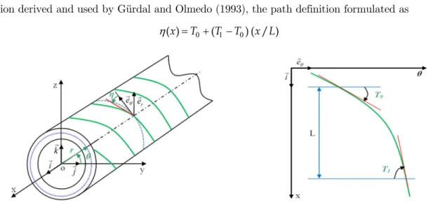
As showed in Figure 2, a typical curvilinear fiber starting from an arbitrary reference point with a fiber orientation angle T0and moving along the x axis, until the fiber orientation angle reaches a value T1 at a characteristic distance L from the reference point. With linear fiber orientation varia-tion derived and used by Gürdal and Olmedo (1993), the path definivaria-tion formulated as
( )x T(TT) ( / )x L (7)
In which η denotes the ply-angle measured from the positive -axis toward the positive x -coordinate in Figure 2. Using this definition, the vector of design variables is | Where T0 and T1 are the fiber orientation angle at the root and tip cross sections which can have values between 0° and 180°. So the two design variables in each layer n are required to determine the variation of the fiber orientation on the surface of the shaft. Therefore the equation (4) becomes as follows:
cos ( ) sin ( ) ( )sin ( )cos ( )
( )sin ( )cos ( ) ( )sin ( )cos ( )
[ ( )]sin ( )cos ( ) (sin ( ) cos ( ))
sin ( )
C C x C x C C x x
C C C C x x C C C x x
C C C C C x x C x x
C C x
Ccos( )x
(8)
2.3 Hierarchical Beam Element Formulation
The spinning flexible shaft is descretized by one hierarchical beam element with two nodes 1 and 2. The element’s nodal degrees of freedom at each node are U ,V,W , x, yand. The local and non-dimensional co-ordinates are related by x L with ∈ , .
The vector displacement formed by the variables U,V,W, x, yand can be written as
, , , , ,U V W
y x
x x y y
p p p
U U m m V V m m W W m m
mp m p m p
x xm m y ym m m m
m m m
U N q x t f V N q y t f W N q z t f
N q t f N q t f N q t f
(9)
And
, , , x, y, U, V, W, x, y,
U V V p p p p p p
N f f f
(10)
Where pU , pV ,pW ,px, py and pare the numbers of hierarchical terms of displacements (are
the numbers of shape functions of displacements). In this work,
x y
U V W
p p p p p p p
The vector of generalized coordinates given by
q
qU,q qV, W,qx,qy,q
T (11)Where
, , ,...., exp , , , ,...., exp ,
, , ,...., exp , , , ,...., exp ,
, , ,...., exp , , , ,...., exp
U V
W x px
y p y
T T
U p V p
T T
W p x x x x
T T
y y y y p
q x x x x j t q y y y y j t
q z z z y j t q j t
q j t q j t
(12)
f,f,fr sin r ; rr ; r , , , .... (13)The functions (f1, f2) are those of the finite element method necessary to describe the nodal
dis-placements of the element; whereas the trigonometric functions fr+2 contribute only to the internal
field of displacement and do not affect nodal displacements. The most attractive particularity of the trigonometric functions is that they offer great numerical stability. The shaft is modeled by one element called hierarchical finite element with p shape functions.
By modelling of the spinning composite shaft by the p- version of the finite element method and applying the Euler-Lagrange equations, the equations of motion of free vibration of spinning flexible shaft can be obtained.
M q
G q
K q
(14)[M] and [K] are the mass and stiffness matrix, [G] is the gyroscopic matrix. The different matrices of the system of equation are given in Appendix.
3 NUMERICAL RESULTS
In this work, we expose the results obtained by our computer code for various applications. Con-vergence towards the solutions is studied by increasing the numbers of shape functions of displace-ments. In the absence of data on vibrations of spinning composite shafts with curvilinear fibers, the formulation is verified by comparisons with published data on spinning composite shafts reinforced by straight fibers. A study of the influence of mechanical and geometrical parameters, boundary conditions and the curvilinear fiber paths on the natural frequencies of the spinning composite shafts with variable stiffness. After the convergence study, in all studied examples, we takes p =10.
3.1 Convergence
The mechanical properties of boron-epoxy are (Bert and Kim, 1995) E11 = 211.0 GPa, E22 = 24.1
GPa, G12 = G23 = 6.9 GPa, 12 = 0.36, ρ= 1967.0 Kg/m3. The shaft has a total length L of 2.47 m.
The mean diameter D and the wall thickness e of the shaft are 12.69 cm and 1.321 mm respectively. The shaft has three layers of equal thickness with curvilinear fibers [<15°|30°>,<45°|60°>,<75°|90°>] starting from the inside surface of the hollow shaft. A shear cor-rection factor ks of 0.503 is also used and the rotating speed Ω =0. In this example, the boron -epoxy spinning shaft is modeled by one element of length L.
The results of the three bending modes for various boundary conditions of the composite shaft with variable stiffness as a function of the number of hierarchical terms p are shown in Figure 3. Figure clearly shows that rapid convergence from above to the solutions occurs as the number of hierarchical terms is increased. This shows the exactitude of the method even with one element and a reduced number of the shape functions. It is noticeable in the case of low frequencies, a very small
3.2 Validation
In the absence of publications of vibration analysis of spinning composite shafts with curvilinear fibers, this model is validated by calculating the critical speeds of spinning composite shafts with straight fibers.
In the following example already treated in our publication (Boukhalfa et al., 2008), the critical speeds of composite shaft for different lamination angles η are analysed and compared with those available in the literature to verify the present model. In this example, the composite hollow shaft made of graphite-epoxy laminae, which are considered by Bert and Kim (1995), are investigated. The mechanical and geometrical properties of this shaft are: E11 = 139.0 GPa, E22 = 11.0 GPa, G12
= 6.05 GPa, G23 =3.78 GPa , 12 = 0.313, ρ= 1578.0 Kg/m3, L =2.47 m, D = 12.69 cm, e = 1.321
mm, 10 layers with straight fibers [90°/45°/-45°/0°6/90°] of equal thickness starting from the inside
surface of the hollow shaft, ks = 0.503.
The shaft is modeled by one element. The shaft is simply-supported at the ends. In this valida-tion, p =10. The results are listed in Table 1. The results from the present model are compatible to that of continuum based Timoshenko beam theory of Chang et al. (2004). In this reference, the supports are flexible and the shaft is modeled by 20 finite elements of equal length (h-version of finite element method (FEM)). But in our application the supports are rigid and the shaft is mod-eled by only one element with two nodes. In this example, is not noticeable the difference between shaft bi-supported on rigid supports or elastic supports because the stiffness of the supports are very large, 1740 GN/m for each support. The rapid convergence while taking only one element and a reduced number of shape functions shows the advantage of the method used. We should stress here that the present model is not only applicable to the thin-walled composite shafts as studied above, but also to the thick-walled shafts as well as to the solid ones.
Theory or Method Lamination angleη[°]
0 15 30 45 60 75 90
Bert and Kim (1995)
Sanders shell. 5527 4365 3308 2386 2120 2020 1997
Bernoulli- Euler beam. 6425 5393 4269 3171 2292 1885 1813
Bresse-Timoshenko beam. 6072 5209 4197 3143 2278 1874 1803
Chang et al. (2004)
Continuum based Timoshenko beam
by the h-version of FEM. 6072 5331 4206 3124 2284 1890 1816
Present Timoshenko beam by the p- version
of FEM. 6094 5359 4222 3129 2284 1890 1816
Table 1: Critical speeds [rpm] of the graphite-epoxy shaft for various lamination angles.
3.3 Results and Discussions
3.3.1 Influence of Gyroscopic Effect on the Natural Frequencies
the boron- epoxy spinning shaft for different boundary conditions is shown in Figure 4. The Camp-bell diagram for the first three bending modes of the boron- epoxy spinning shaft bi- simply sup-ported (S-S) is shown in Figure 5.
The gyroscopic effect inherent to spinning structures induces a precession motion. The forward modes (F) increase with increasing rotating speed however the backward modes (B) decrease. This effect has a significant influence on the behaviors of the spinning shafts. The numerical results of these figures are given in tables 2 and 3 to show this influence of the gyroscopic effect.
Figure 3: Convergence of the natural frequency ω for the three bending modes of the boron-epoxy shaft with variable stiffness [<15°|30°>,<45°|60°>,<75°|90°>] for different boundary conditions
(S: simply-supported; C: clamped) as a function of the number of hierarchical terms p.
Rotating speed Ω
[rad/s]
Frequency ω1 [Hz]
1B (S-S) 1F (S-S) 1B (C-C) 1F (C-C) 1B (C-S) 1F (C-S)
0 65.6539 65.6539 145.1298 145.1298 102.6872 102.6872
100 65.6046 65.7032 145.0773 145.1822 102.6320 102.7425
200 65.5554 65.7525 145.0249 145.2347 102.5767 102.7978
300 65.5062 65.8018 144.9725 145.2872 102.5215 102.8532
400 65.4571 65.8512 145.3397 145.3397 102.4663 102.9085
500 65.4080 65.9006 144.8676 145.3921 102.4111 102.9639
600 65.3589 65.9501 144.8152 145.4446 102.3559 103.0193
700 65.3098 65.9996 144.7628 145.4971 102.3008 103.0747
800 65.2608 66.0491 144.7104 145.5497 102.2457 103.1301
900 65.2118 66.0986 144.6580 145.6022 102.1906 103.1855
1000 65.1629 66.1482 144.6056 145.6547 102.1355 103.2410
Table 2: The first bending mode of the boron- epoxy shaft with variable stiffness [<15°|30°>,<45°|60°>,<75°|90°>] for different boundary conditions and various rotating speed Ω(S: simply-supported; C: clamped).
ω|
Hz
]
p
Rotating speed Ω
[rad/s]
Frequency ω [Hz]
1B (S-S) 1F (S-S) 2B (S-S) 2F (S-S) 3B (S-S) 3F (S-S)
0 65.6539 65.6539 252.9123 252.9123 537.8773 537.8773
100 65.6046 65.7032 252.7413 253.0835 537.5647 538.1899
200 65.5554 65.7525 252.5703 253.2547 537.2522 538.5026
300 65.5062 65.8018 252.3993 253.4260 536.9397 538.8152
400 65.4571 65.8512 252.2284 253.5974 536.6272 539.1279
500 65.4080 65.9006 252.0577 253.7688 536.3147 539.4407
600 65.3589 65.9501 251.8869 253.9403 536.0022 539.7534
700 65.3098 65.9996 251.7163 254.1119 535.6898 540.0662
800 65.2608 66.0491 251.5457 254.2835 535.3774 540.3790
900 65.2118 66.0986 251.3752 254.4552 535.0651 540.6918
1000 65.1629 66.1482 251.2048 254.6270 534.7528 541.0046
Table 3: The first three of bending modes of the boron- epoxy shaft bi- simply supported (S-S) with variable stiffness [<15°|30°>,<45°|60°>,<75°|90°>] for different rotating speed Ω.
Figure 4: Campbell diagram for the first bending mode of the boron- epoxy shaft with variable stiffness [<15°|30°>,<45°|60°>,<75°|90°>] for different boundary conditions (S: simply-supported; C: clamped).
ω1
[H
z]
Ω [rpm]
Figure 5: Campbell diagram for the first three of bending modes of the boron- epoxy shaft bi- simply supported (S-S) with variable stiffness [<15°|30°>,<45°|60°>,<75°|90°>].
Figure 6: Campbell diagram for the bending fundamental frequency ω1of the carbon- epoxy shaft
with variable stiffness [< 5°| °>] bi-simply supported.
ω[
Hz
]
Ω [rpm]
B S‐S F S‐S B S‐S F S‐S B S‐S F S‐S
ω1
[Hz]
Ω |rpm]
3.3.2. Influence of the fibers orientations on the natural frequencies
In order to show the effects of the fibers orientations on the natural frequencies, a carbon-epoxy spinning shafts are bi- simply-supported (S-S). The physical properties of material (Singh and Gup-ta, 1996) are: E11 = 130. GPa, E22 = 10. GPa, G12 = G23 = 7. GPa, 12 = 0.25, ρ= 1500. Kg/m3.
The geometric parameters are L =1.0 m, D = 0.1 m, e = 4 mm, single layer with curvilinear fibers [< | >], and ks= 0.503. We fix T0 =15° and we change T1.
Figure 6 shows the variation of the bending fundamental frequency ω1according to the rotating speeds Ω for various curvilinear fibers [< 5°| >]. According to these results, the first bending fre-quencies of the composite shaft decrease when T1 angle increases and vice versa.
3.3.3 Influence of the stacking sequence on the natural frequencies
By considering the same preceding carbon- epoxy spinning shaft but we change the fiber orienta-tions. In order to show the permutation effects of the fibers orientations on the natural frequencies, we consider the following permutations for one and two then for three layers of equal thickness starting from the inside surface of the hollow shaft:
First permutation between two angles for single curvilinear fibers in the same layer to have [<15°|75°>] and [<75°|15°>];
Second permutation between two curvilinear fibers to have [<15°|75°>,[<45°|60°>] and [<45°|60°>,[<15°|75°>];
Third permutation between three curvilinear fibers to have [<15°|75°>,<45°|60°>,<30°|90°>] , [<45°|60°>,<15°|75°>,<30°|90°>] and [<30°|90°>,<45°|60°>,<15°|75°>].
Figure 7: Campbell diagram for the bending fundamental frequency ω1of the carbon- epoxy shaft
with variable stiffness bi-simply supported for different permutations of fiber orientations.
ω1
[Hz
]
Ω [rpm]
B [< °| °>] F [< °| °>]
B [< °| °>] F [< °| °>]
Figure 7 shows the Campbell diagram for the bending fundamental frequency of the carbon- epoxy shaft bi-simply supported (S-S) with variable stiffness for different permutations of fiber ori-entations.
It is found that the first natural frequencies are almost the same if we permute the angles T0 and T1in the same layer [<T0| T1>] and [<T1| T0>].
It is found that the first natural frequencies are very close if we permute two adjacent layers: [< | >, < | >] and [< | >, < | >] for two layers;
[< | >, < | >,< | >] and [< | >, < | >,< | >] for three layers.
In order to show the symmetric, anti-symmetric and unsymmetric effects of the fibers orienta-tions on the natural frequencies, we consider the following stackings for three then for four layers of equal thickness starting from the inside surface of the hollow shaft.
For three layers, we use three fiber orientations <30°|60°>,<45°|60°> and -<45°|60°> to combine various stackings:
Two symmetric lay-up [<45°|60°>,<30°|60°>,<45°|60°>] and [<30°|60°>, <45°|60°>,<30°|60°>];
Two anti-symmetric lay-up [-<45°|60°>,<30°|60°>,<45°|60°>] and [<45°|60°>,<30°|60°>,-<45°|60°>];
Two unsymmetric lay-up [<45°|60°>,<45°|60°>,<30°|60°>] and [<30°|60°>,<30°|60°>,<45°|60°>].
Figure 8: Campbell diagram for the bending fundamental frequency ω1of the carbon- epoxy shaft
bi-simply supported with symmetric, anti-symmetric and unsymmetric stackings (three layers).
ω1
[Hz]
Ω [rpm]
Figure 8 shows the Campbell diagram for the bending fundamental frequency ω1of the carbon- epoxy shaft bi-simply supported (S-S) with symmetric, anti-symmetric and unsymmetric stackings for three layers.
It is found that the first natural frequencies of spinning shafts which have anti-symmetric stack-ings are very close [-< | >, < | >,< | >] and [< | >, < | >,-< | >].
It is found that the first natural frequencies of spinning shafts which have symmetric stackings are a little close [< | >, < | >,< | >] and [< | >, < | >,-< | >].
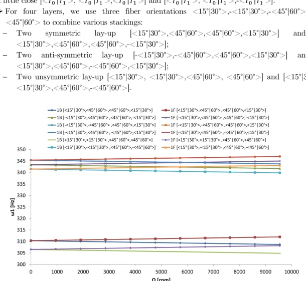
For four layers, we use three fiber orientations <15°|30°>,-<15°|30°>,-<45°|60°> and <45°|60°> to combine various stackings:
Two symmetric lay-up [<15°|30°>,<45°|60°>,<45°|60°>,<15°|30°>] and [-<15°|30°>,<45°|60°>,<45°|60°>,-<15°|30°>];
Two anti-symmetric lay-up <15°|30°>,-<45°|60°>,<45°|60°>,<15°|30°>] and [-<15°|30°>,<45°|60°>,-<45°|60°>,<15°|30°>];
Two unsymmetric lay-up [<15°|30°>, <15°|30°>,<45°|60°>, <45°|60°>] and [<15°|30°>,-<15°|30°>,<45°|60°>,-<45°|60°>].
Figure 9: Campbell diagram for the bending fundamental frequency ω1of the carbon- epoxy shaft
bi-simply supported with symmetric, anti-symmetric and unsymmetric stackings (four layers).
Figure 9 shows the Campbell diagram for the bending fundamental frequency ω1of the carbon- epoxy shaft bi-simply supported (S-S) with symmetric, anti-symmetric and unsymmetric stackings for four layers.
It is found that the first natural frequencies of spinning shafts which have anti-symmetric stack-ings are very close [< | >, < | >, < | >,< | >] and [-< | >, < | >,< | >,-< | >].
ω1
[H
z]
Ω [rpm]
It is found that the first natural frequencies of spinning shafts which have symmetric stackings are a little close [-< | >, -< | >,< | >,< | >] and [-< | >, < | >,-< | >,< | >].
It is found that the first natural frequencies of spinning shafts which have unsymmetric stack-ings are far.
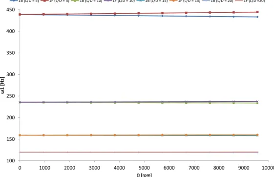
3.3.4 Influence of the Ratios L/D and e/D on the Natural Frequencies
In Figure 10, the variation of the bending fundamental frequency ω1 of the carbon-epoxy shaft bi-simply supported as a function of rotating speed Ω (Campbell diagram) for various ratios L/D. It is the same spinning shaft used previously but we change the fiber orientations at six layers of equal thickness with curvilinear fibers [∓<15°|75°>,∓<45°|60°>,∓<30°|90°>] i.e. [ <15°|75°>, <15°|75°>, <45°|60°>, <45°|60°>, <30°|90°>, <30°|90°>] starting from the inside surface of the hollow shaft (L =1m).
It is noted, if ratio L/D increases the first natural frequencies decreases and vice versa. For more details you can see our publication (Boukhalfa and Hadjoui, 2010).
In Figure 11, the variation of the bending fundamental frequency ω1 of the carbon-epoxy spin-ning shaft bi-simply supported as a function of rotating speed Ω (Campbell diagram) for various ratios e/D. It is the same spinning shaft used previously (D =0.1m).
In spite of the change of the e/D ratio, the first natural frequencies are slightly increased. This is due to the deformation of the cross section is negligible, and thus natural frequencies of the thin-walled shaft would approximately independent of thickness ratio e/D.
Figure 10: Campbell diagram for the bending fundamental frequency ω1of the carbon- epoxy
shaft bi-simply supported for various ratios L/D.
ω1 [
Hz
]
Ω [rpm]
Figure 11: Campbell diagram for the bending fundamental frequency ω1of the carbon- epoxy
spinning shaft bi-simply supported for various ratios e/D.
4 CONCLUSIONS
The free vibrations analysis of spinning composite shafts with curvilinear fibers using the p-version of finite element method with trigonometric shape functions is presented in this analysis. In the absence of data on vibrations of spinning composite shafts with curvilinear fibers, the formulation is verified by comparisons with published data on spinning composite shafts reinforced by straight fibers.The results obtained agree with those available in the literature. Several examples were treat-ed to determine the influence of the various geometrical and mechanical parameters of the spinning shafts on natural frequencies. This work use led to obtain at the following conclusions
Monotonous and uniform convergence is checked by increasing the number of the shape func-tions p. The convergence of the solutions is ensured by the element beam with two nodes. The results agree with the solutions found in the literature.
The gyroscopic effect causes a coupling of orthogonal displacements to the axis of rotation, and by consequence separates the frequencies in two branches, backward (B) and forward (F) precession modes. In all cases the forward modes increase with increasing rotating speed how-ever the backward modes decrease. This effect has a significant influence on the behaviors of the spinning shafts.
The first natural frequencies of the thin-walled spinning composite shaft are approximately independent of the thickness ratio and mean diameter of the shaft.
The first bending natural-frequencies of the spinning composite shafts are influenced appre-ciably by changing the ply angle η (x) of curvilinear fibers, the stacking sequence, the length, the mean diameter, the materials, the rotating speed and the boundary conditions.
ω1
[Hz]
Ω [rpm]
If we combine the same fiber orientations to form various stackings, we find:
(a) The first bending natural-frequencies are almost the same if we permute the angles T0 and
T1in the same layer and are very close if we permute two adjacent layers.
(b) The first bending natural-frequencies of spinning shafts which have anti-symmetric stack-ings are very close and are a little close which have symmetric stackstack-ings.
(c) The first bending natural-frequencies of spinning shafts which have unsymmetric stackings are far.
Prospects for studies which can be undertaken following this work: Curvilinear fiber optimiza-tion of a spinning composite shaft.
References
Abdalla, M.M., Setoodeh, S., Gürdal, Z. (2007). Design of variable stiffness composite panels for maximum funda-mental frequency using lamination parameters. Composite Structures 81(2): 283-291.
Bert, C.W., Kim, C.D. (1995). Whirling of composite-material driveshafts including bending, twisting coupling and transverse shear deformation. Journal of Vibration and Acoustics 117: 17-21
Berthelot, J.M. (1996). Matériaux Composites, Comportement Mécanique et Analyse des Structures, Masson, Paris, Deuxième édition.
Blom, A.W., Setoodeh, S., Hol, J., Gürdal, Z. (2008).Design of variable-stiffness conical shells for maximum funda-mental Eigen frequency. Computers and Structures 86(9): 870–878.
Blom, A.W., Stickler, P.B., Gürdal, Z. (2010). Optimization of a composite cylinder under bending by tailoring stiff-ness properties in circumferential direction. Composites Part B: Engineering 41(2): 157-165.
Boukhalfa, A. (2014). Dynamic analysis of a spinning functionally graded material shaft by the p-version of the finite element method. Latin American Journal of Solids and Structures 11: 2018-2038
Boukhalfa, A., Hadjoui, A. (2010). Free vibration analysis of an embarked rotating composite shaft using the hp -version of the FEM. Latin American Journal of Solids and Structures 7: 105–141
Boukhalfa, A., Hadjoui, A., Hamza Cherif, S.M. (2008). Free vibration analysis of a rotating composite shaft using the p-version of the finite element method. International Journal of Rotating Machinery. Article ID 752062, 10 pages. Chang, M.Y., Chen, J.K., Chang, C.Y. (2004). A simple spinning laminated composite shaft model. International Journal of Solids and Structures 41: 637–662.
Dharmarajan, S., McCutchen Jr., H. (1973). Shear coefficients for orthotropic beams. Journal of Composite Materials 7: 530–535.
DiNardo, M.T., Lagace, P.A. (1989). Buckling and postbuckling of laminated composite plates with ply drop-offs.
AIAA journal 27(10): 1392–1398.
Gürdal, Z., Olmedo R. (1993). In-plane response of laminates with spatially varying fiber orientations-variable stiff-ness concept. AIAA journal 31(4): 751–758.
Gürdal, Z., Olmedo, R. (1992). Composite laminates with spatially varying fiber orientations: variable stiffness panel concept. Proceedings of the AIAA/ASME/ASCE/AHS/ASC 33rd structures, structural dynamics and materials conference (2): 798–808.
Gürdal, Z., Tatting, B.F., Wu, K.C. (2005).Tow-placement technology and fabrication issues for laminated compo-site structures. Proceedings of the 46th AIAA/ASME/ASCE/AHS/ASC Structures, Structural Dynamics and Mate-rials (SDM) Conference, Austin TX.
Hyer, M., Charette, R. (1991). Use of curvilinear fiber format in composite structure design. AIAA journal, vol. 29(6):1011–1015.
Hyer, M., Lee, H. (1991). The use of curvilinear fiber format to improve buckling resistance of composite plates with central circular holes. Composite Structures 18(3): 239-261.
Khani, A., IJsselmuiden, S., Abdalla, M., Gürdal, Z. (2011). Design of variable stiffness panels for maximum strength using lamination parameters. Composites Part B: Engineering 42(3): 546-552.
Leissa, A., Martin, A. (1990). Vibration and buckling of rectangular composite plates with variable fiber spacing. Composite Structures 14(4): 339–357.
Marouene, A. (2015). Résistance à la compression et au flambage des composites carbone/époxy à rigidité variable fabriqués par le procédé de placement automatique des fibres, Ph.D. Thesis (in French), Montreal University, Mon-treal Polytechnic, Canada.
Nik, MA., Fayazbakhsh, K., Pasini, D., Lessard, L. (2012). Surrogate-based multi-objective optimization of a compo-site laminate with curvilinear fibers. Compocompo-site Structures 94(8): 2306-2313.
Olmedo, R., Gürdal, Z. (1993). Buckling response of laminates with spatially varying fiber orientations. Proceedings of the AIAA/ASME/ASCE/AHS/ASC 34th Structures, Structural Dynamics, and Materials Conference (1): 2261– 2269.
Ribeiro, P. (2015a). Non-linear modes of vibration of thin cylindrical shells in composite laminates with curvilinear fibres. Composite Structures 122: 184–197
Ribeiro, P. (2015b). Linear modes of vibration of cylindrical shells in composite laminates reinforced by curvilinear fibres. Journal of Vibration and Control: 1–18.
Ribeiro, P., Akhavan, H. (2012). Non-linear vibrations of variable stiffness composite laminated plates. Composite Structures 94(8): 2424-2432.
Ribeiro, P., Akhavan, H., Teter, A., Warmiński, J. (2014). A Review on the mechanical behaviour of curvilinear fibre composite laminated panels. Journal of Composite Materials 48(22): 2761–2777.
Rouhi, M., Ghayoor, H., Hoa, S.V., Hojjati, M. (2015). Multi-objective design optimization of variable stiffness com-posite cylinders. Comcom-posites Part B: Engineering 69: 249-255.
Singh, S.E., Gupta, K. (1996). Composite shaft rotordynamic analysis using a layerwise theory. Journal of Sound and Vibration 191(5):739–756
Tatting, B.F. (1998). Analysis and design of variable stiffness composite cylinders. Ph.D. Thesis, Virginia Polytech-nic Institute and State University, USA.
Venkatachari, A., Natarajan, S., Haboussi, M., Ganapathi, M. (2016). Environmental effects on the free vibration of curvilinear fibre composite laminates with cutouts. Composites Part B 88: 131-138.
Waldhart, C. (1996). Analysis of tow-placed, variable-stiffness laminates. Ph.D. Thesis, Virginia Polytechnic Insti-tute and State University, USA.
Wu, Z., Weaver, PM., Raju, G. (2013). Postbuckling optimisation of variable angle tow composite plates. Composite Structures 103: 34-42.
Yazdani, S., Ribeiro, P. (2015). A layerwise p-version finite element formulation for free vibration analysis of thick composite laminates with curvilinear fibres. Composite Structures 120: 531–542
NOMENCLATURE
U(x, y, z) Displacement in x direction. V(x, y, z) Displacement in y direction. W(x, y, z) Displacement in z direction.
x Rotation angles of the cross-section about the y axis. y Rotation angles of the cross-section, about the z axis.
Angular displacement of the cross-section due to the torsion deformation of the shaft.
E Young modulus.
G Shear modulus.
(1, 2, 3) Principal axes of a layer of laminate
i e, r,e
Axes of cylindrical coordinates.
i , ,j k
Axes of Cartesian coordinates. (x, y, z) Cartesian coordinates.(x, r, θ) Cylindrical coordinates. Cij’, Cij Elastic constants.
ks Shear correction factor.
Poisson coefficient.
ρ Masse density.
L Length of the shaft. D Mean radius of the shaft. e Wall thickness of the shaft.
Rn The nth layer inner radius of the composite shaft.
Rn+1 The nth layer outer radius of the composite shaft.
k Number of the layer of the composite shaft.
η(x) Lamination angle of curvilinear fibers.
θ Circumferential coordinate.
Local and non-dimensional co-ordinates.
ω Natural frequency
Ω Rotating speed.
[N] Matrix of the shape functions.
f ( ) Shape functions.
p Number of the shape functions or number of hierarchical terms.
t Time.
Ec Kinetic energy.
Ed Strain energy.
{qi} Generalized coordinates, with (i = U, V, W,x,y, )
[M] Masse matrix. [K] Stiffness matrix. [G] Gyroscopic matrix.
APPENDIX
The various matrices of the equation (14) as follows:
x y U V W M M M M M M M ;
x y U V W T TT T T
T
K K
K K K
K K K
K K K K K
K K K K
K K (A1-2)
T G G G ;
TU m U U
M I L N N d ;
TV m V V
M I L N N d (A3-4-5)
TW m W W
M I L N N d ;
1
0
x x x
T
d
M I L N N d
;
y
y yT d
M I L N N d (A6-7-8)
M I Lp
N T N d ;
TU U U
K A N N d
L ;
( ) TV s V V
K k A A N N d
L (A9-10-11)
( ) TW s W W
K k A A N N d
L ;
s
T UK k A N N d
L (A12-13)
xT
s V
K k A N N d
L ;
( ) y T s VK k A A N N d (A14-15)
( ) x T s WK k A A N N d ;
yT
s W
K k A N N d
L (A16-17)
y x
x y T T
s s
K k A N N d k A N N d ;
K k Bs
N T N dL (A18-19)
( ) x x x x x
T T
s
K B N N d Lk A A N N d
L ;
x y T pG I L N N d (A20-21)
( )y y y y y
T T
s
K B N N d Lk A A N N d
L (A22)
The terms of the matrices are a function of the integrals:
mn m n
![Table 1: Critical speeds [rpm] of the graphite-epoxy shaft for various lamination angles](https://thumb-eu.123doks.com/thumbv2/123dok_br/18887253.424112/7.808.38.734.620.827/table-critical-speeds-graphite-epoxy-various-lamination-angles.webp)
![Table 2: The first bending mode of the boron- epoxy shaft with variable stiffness [<15°|30°>,<45°|60°>,<75°|90°>]](https://thumb-eu.123doks.com/thumbv2/123dok_br/18887253.424112/8.808.93.757.692.960/table-bending-mode-boron-epoxy-shaft-variable-stiffness.webp)
![Figure 4: Campbell diagram for the first bending mode of the boron- epoxy shaft with variable stiffness [<15°|30°>,<45°|60°>,<75°|90°>] for different boundary conditions (S: simply-supported; C: clamped)](https://thumb-eu.123doks.com/thumbv2/123dok_br/18887253.424112/9.808.51.719.105.395/figure-campbell-variable-stiffness-different-boundary-conditions-supported.webp)
![Figure 5: Campbell diagram for the first three of bending modes of the boron- epoxy shaft bi- simply supported (S-S) with variable stiffness [<15°|30°>,<45°|60°>,<75°|90°>]](https://thumb-eu.123doks.com/thumbv2/123dok_br/18887253.424112/10.808.128.720.92.460/figure-campbell-diagram-bending-simply-supported-variable-stiffness.webp)
![Figure 6 shows the variation of the bending fundamental frequency ω 1 according to the rotating speeds Ω for various curvilinear fibers [< 5 ° | >]](https://thumb-eu.123doks.com/thumbv2/123dok_br/18887253.424112/11.808.70.721.453.946/figure-variation-bending-fundamental-frequency-according-rotating-curvilinear.webp)