Notably improved inversion of Differential Mobility Particle Sizer data obtained under conditions of fluctuating particle number concentrations

(1)

AMTD

8, 10283–10317, 2015

Notably improved DMPS data inversion

B. Mølgaard et al.

Title Page

Abstract Introduction

Conclusions References

Tables Figures

◭ ◮

Back Close

Full Screen / Esc

Printer-friendly Version Interactive Discussion

Discussion

P

a

per

|

Discussion

P

a

per

|

Discussion

P

a

per

|

Discussion

P

a

per

|

Atmos. Meas. Tech. Discuss., 8, 10283–10317, 2015 www.atmos-meas-tech-discuss.net/8/10283/2015/ doi:10.5194/amtd-8-10283-2015

This discussion paper is/has been under review for the journal Atmospheric Measurement Techniques (AMT). Please refer to the corresponding final paper in AMT if available.

Notably improved inversion of Di

_ff

erential

Mobility Particle Sizer data obtained

under conditions of fluctuating particle

number concentrations

B. Mølgaard1, J. Vanhatalo2, P. P. Aalto1, N. L. Prisle1, and K. Hämeri1

1

Department of Physics, University of Helsinki, Helsinki, Finland

2

Department of Environmental Sciences, University of Helsinki, Helsinki, Finland

Received: 9 June 2015 – Accepted: 4 September 2015 – Published: 7 October 2015

Correspondence to: B. Mølgaard ([email protected])

(2)

AMTD

8, 10283–10317, 2015

B. Mølgaard et al.

Title Page

Tables Figures

◭ ◮

Back Close

Full Screen / Esc

Discussion

P

a

per

|

Discussion

P

a

per

|

Discussion

P

a

per

|

Discussion

P

a

per

|

Abstract

The Differential Mobility Particle Sizer (DMPS) is designed for measurements of parti-cle number size distributions. It performs a number of measurements while scanning over different particle sizes. A standard assumption in the data processing (inversion) algorithm is that the size distribution remains the same throughout each scan. For a 5

DMPS deployed in an urban area this assumption is likely to be violated most of the time, and the resulting size distribution data are unreliable. To improve the reliability, we developed a new algorithm using a statistical model in which the problematic assump-tion was replaced with more realistic smoothness assumpassump-tions, which were expressed through Gaussian Process prior probabilities. We tested the model with data from a 10

twin-DMPS located in Helsinki and found that it provides size distribution data which are much more realistic. Furthermore, particle number concentrations extracted from the DMPS data were compared with data from a condensation particle counter at 30 s resolution, and the overall agreement was good. Thus, the quality of the inverted data was clearly improved.

15

1 Introduction

There is no direct way of measuring the size distribution of fine particles. To get informa-tion on the size distribuinforma-tion, mobility particle size spectrometers (Wiedensohler et al., 2012) select in turns particles of various electrical mobilities, and for each electrical mobility the number of particles in some volume is counted. To obtain the size distri-20

butions the dependence of electrical mobilities on particle sizes is utilised. However, the electrical mobility depends also on the particle charge, so various combinations of particle size and charge give the same electrical mobility, and the inference of the actual particle size distribution is not trivial. The algorithms which have been developed for this purpose are generally known as inversion algorithms. The task can be split into 25

(3)

probabili-AMTD

8, 10283–10317, 2015

B. Mølgaard et al.

Title Page

Tables Figures

◭ ◮

Back Close

Full Screen / Esc

Discussion

P

a

per

|

Discussion

P

a

per

|

Discussion

P

a

per

|

Discussion

P

a

per

|

ties of particles in the sampled air, and the actual inversion. In this study we focused on the latter part. Further we restrict ourselves to considering Differential Mobility Par-ticles Sizers (DMPS) which differ from Scanning Mobility Particle Sizers (SMPS) by changing the selected electrical mobility in discrete steps.

A DMPS typically performs a few tens of measurements while scanning over a wide 5

range of electrical mobilities. Each measurement takes several seconds and a typical waiting time between the measurements is around 10 s. Thus, each scan takes 5 to 10 min. The inversion must be based on some assumption about the time evolution of the aerosol during the scan. The simplest and most commonly used assumption is that the particle size distribution stays constant during each scan. In remote areas, where 10

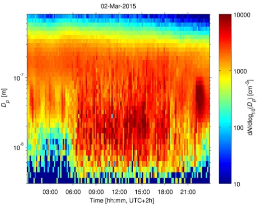
the particle size distribution changes slowly most of the time, this assumption is rea-sonable most of the time. However, when a DMPS is deployed in a city with numerous nearby sources and a turbulent wind flow, this assumption is often far from the truth, and many of the derived particle size distributions are unreliable. Let us illustrate this with an example using inverted data from the twin-DMPS (comprises two DMPSs) at 15

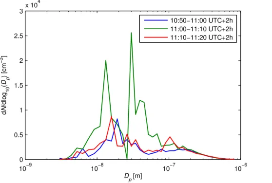
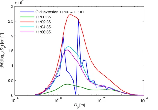
the SMEAR III station in Helsinki (Järvi et al., 2009) on 2 March 2015. The particle size distribution fluctuated substantially during daytime (Fig. 1) but at night time there were periods without fluctuations. For these night time periods, the particle size distribution was a rather smooth function of size, but at daytime unrealistically narrow peaks are present in the inverted data. In particular, the scan from 11:00 to 11:10 UTC+2 h is 20

problematic, because of the strong, narrow peaks at 13 and 30 nm (Fig. 2). Single-charged particles of these two sizes are measured almost simultaneously in the two DMPSs, so the peaks at these sizes are most likely caused by a brief concentration peak. At 26 nm dN/dlog10Dpappears to be low (Fig. 2), although the raw data indicate that the concentration was already elevated when the DMPS measured particles at 25

(4)

AMTD

8, 10283–10317, 2015

B. Mølgaard et al.

Title Page

Tables Figures

◭ ◮

Back Close

Full Screen / Esc

Discussion

P

a

per

|

Discussion

P

a

per

|

Discussion

P

a

per

|

Discussion

P

a

per

|

measurement belonged to the 30 nm bin. Additionally, double-charged 39 nm particles contributed somewhat to the particle count. As a result, a small value was assigned to dN/dlog10Dpat 26 nm.

A few studies have addressed this issue of possible size distribution changes hap-pening during a scan. Voutilainen and Kaipio (2001) presented an algorithm based 5

on the Kalman filter. They let the particle size distribution change in discrete steps at each measurement based on the observation and a random walker. Subsequently, a smoother and a non-negativity constraint was applied. The algorithm was applied to synthetic data, and it reproduced a slowly varying size distribution well. Voutilainen and Kaipio (2002, 2005) parametrised the size distribution and replaced the random walker 10

by estimations of the time evolution based on an aerosol model which took coagulation and condensation into account. The underlying assumption is that the DMPS continu-ously samples from the same aerosol which changes in time due to these processes. Also this assumption is generally invalid in a city. Although, the algorithm by Vouti-lainen and Kaipio (2005) was also shown to adjust to abrupt changes in the aerosol 15

within a couple of minutes, it was not designed for use in urban locations.

In this work, we developed a new inversion algorithm for processing DMPS data from locations with fluctuating particle number concentrations. The particle number size distribution was modelled as function of time and particle size using a Gaussian Process (GP) model (Rasmussen and Williams, 2006). Assumptions of smoothness in 20

both dimensions were incorporated through a GP prior. We tested our new algorithm with data from the twin-DMPS at the urban background station SMEAR III in Helsinki. For periods with considerable fluctuations, the time resolution and the reliability of the derived particle number size distribution was substantially improved. A demo version of our algorithm is provided in the Supplement.

(5)

AMTD

8, 10283–10317, 2015

B. Mølgaard et al.

Title Page

Tables Figures

◭ ◮

Back Close

Full Screen / Esc

Discussion

P

a

per

|

Discussion

P

a

per

|

Discussion

P

a

per

|

Discussion

P

a

per

|

2 Methods

2.1 Quantification of particle size distributions

Particle size distributions are usually described by the dN/dlog₁₀Dp, although it is not a distribution function in a mathematical sense. N is the product of the total particle number concentration and the cumulative distribution function of the particle diame-5

ters (Hinds, 1999). Thus, dN/dlog₁₀Dp is the product of the concentration and the probability density function on the logarithmic scale.

2.2 DMPS

The DMPS comprises a neutraliser (bi-polar charger), a Differential Mobility Analyser (DMA), and a Condensation Particle Counter (CPC). In the neutraliser, ionising radia-10

tion ensures that the particles in the sampled air reach the equilibrium charge distribu-tion. This charge distribution is known and depends on the particle size. In the DMA, the voltage and air flow are adjusted to select particles with a certain electrical mobility

Z= qCc

3πηDp, whereq is the charge,Dpis the mobility (Stokes’) diameter,Cc is the

Cun-ningham slip correction factor, which depends onDp, andηis the dynamic viscosity of 15

the air. SoZ depends on two particle properties:D_pandq=ze, wherezis an integer, and eis the elementary charge. The particles selected by the DMA flow to the CPC which counts them. Usually, the flows are kept constant and the DMPS scans over a few tens of discrete DMA voltages in order to select particles of different electrical mobilities. At each of these voltages, a measurement is performed with the CPC. 20

2.3 Transfer function

(6)

AMTD

8, 10283–10317, 2015

B. Mølgaard et al.

Title Page

Tables Figures

◭ ◮

Back Close

Full Screen / Esc

Discussion

P

a

per

|

Discussion

P

a

per

|

Discussion

P

a

per

|

Discussion

P

a

per

|

– PDMA, the probability that the particle is selected by the DMA (Stolzenburg, 1988; Mamakos et al., 2007),

– PPen, the probability that the particle penetrates all sampling lines without being deposited (Wiedensohler et al., 2012), and

– PCPC, the detection probability for particles reaching the CPC. 5

The DMA is designed to select particles with electric mobilities in a narrow band. The electric mobility depends onD_pand the numberzof charges. The probability of a cer-tain numberz of charges depends on the particle size, i.e. onDp. Thus,PDMA can be described as a function ofD_pand the DMA voltageU. Diffusion is the main reason for deposition of particles in the sampling lines, and the particle diffusivity depends on the 10

particle size, soPPenis also a function ofDp.PCPCis close to unity (1) for most particles, but for the smallest particles it is lower. During a measurementi the DMA voltage is kept at a constant valueU_i. We will defineT_i(D_p)=T(D_p,U_i).T_i has a few clear peaks and is zero on the rest of the interval. The largest peak is for the diameter which gives the selected electrical mobilityZ when the number of chargesz equals 1 or −1. The 15

sign depends on the polarity of the DMA voltage. A second peak is observed for the diameterDp which gives the same electrical mobility for particle with double charge. This peak is smaller than the first one, because particles are less likely to carry two than one charge. Triple charged particles cause a third peak, which is smaller than the second peak, and subsequent peaks are even smaller.

20

2.4 Inversion algorithm based on a GP model

A GP, or Gaussian random field, is a stochastic process that can be used to define prob-ability distributions over functions, and it is a generalisation of the multivariate normal (Gaussian) distribution (O’Hagan, 1978; Rasmussen and Williams, 2006). It is defined by a mean and a covariance function, which determine the properties, such as the 25

(7)

AMTD

8, 10283–10317, 2015

B. Mølgaard et al.

Title Page

Tables Figures

◭ ◮

Back Close

Full Screen / Esc

Discussion

P

a

per

|

Discussion

P

a

per

|

Discussion

P

a

per

|

Discussion

P

a

per

|

to model coloured (spatially correlated) noise in spatial statistics (Gelfand et al., 2010), and they have obtained increasing interest also in, e.g., statistics and machine learning due their good interpolation and smoothing properties as well as convenient marginal-ization and conditioning properties (see Sect. 2.5.2) (Rasmussen and Williams, 2006; Vanhatalo et al., 2010).

5

Let us define a latent functionf(t,u)=log(dN/du), wheret is time andu=log10Dp. We use the Bayesian formalism, and express our prior belief about its smoothness through a GP prior. Thus, the posterior, which is proportional to the product of the prior and the likelihood, is a probability distribution off.

2.4.1 Likelihood function

10

Each measurement i provides a count yi of particles, so the Poisson distribution Poi(y_i_|λ_i)=exp(₋λ_i)λ

yi i

y_i! is suitable for each factor of the likelihood

p(y_|f)=Y

i

exp(−λi)

λyi

i

y_i!. (1)

The rate parameterλ_i is obtained by integrating the product of dN/dlog10Dp and the transfer functionTi. In terms off andudefined above

15

λ_i =Q

∞ Z

−∞ ti,end_Z

ti,begin

exp(f(t,u))T_i(10u)dtdu, (2)

(8)

AMTD

8, 10283–10317, 2015

B. Mølgaard et al.

Title Page

Tables Figures

◭ ◮

Back Close

Full Screen / Esc

Discussion

P

a

per

|

Discussion

P

a

per

|

Discussion

P

a

per

|

Discussion

P

a

per

|

has much shorter duration than a scan), the following approximation holds:

λi ≈Vi ∞ Z

−∞

exp(f(ti,u))Ti(10u)du, (3)

whereV_i is the volume of sampled air, andt_i is the middle of the time interval between

ti,begin and ti,end. Because Ti has a few clear peaks and is zero on the rest of the interval, the integral can be well approximated by a sum. LetT_i,j equal the integral ofT_i

5

over the peak centred at sizeu_i,j and letf_i_,j =f(t_i,u_i,j). Then

λ_i ≈V_iX

j

exp(f_i,j)T_i,j (4)

The number of peaks to consider in this sum depends on the size of the selected parti-cles. When the DMA selects particles with high electrical mobility (meaning very small particles),Ti,2≪Ti,1, because these particles have very small probability of carrying 10

two charges. On the other hand, for particles with diameters of hundreds of nanome-tres, multiple charges are common and we considered particles with up to six charges (following the custom of the old inversion algorithm).

2.4.2 Prior

The particle number size distribution is assumed to be a smooth function of the particle 15

size and it is assumed to vary smoothly over time. These properties are modelled by giving a GP prior for the latent function

f(t,u)_∼GP(µ(t,u),k(u,u′)k(t,t′)) (5)

whereµ(t,u) is the mean function andk(u,u′)k(t,t′) is the covariance function such thatk(u,u′)=Cov(f(t,u),f(t,u′)) andk(t,t′)=Cov(f(t,u),f(t′,u)).

(9)

AMTD

8, 10283–10317, 2015

B. Mølgaard et al.

Title Page

Tables Figures

◭ ◮

Back Close

Full Screen / Esc

Discussion

P

a

per

|

Discussion

P

a

per

|

Discussion

P

a

per

|

Discussion

P

a

per

|

We assume that the mean function is constant,µ(t,u)=µ, so that it represents the average off and give it a Gaussian priorµ∼N(0,σµ2). This implies that the prior can be written asf(t,u)_∼GP(0,σ_µ2+k(u,u′)k(t,t′)). The covariance function along the particle size follows the Matern covariance function with 5/2 degrees of freedom (Rasmussen and Williams, 2006)

5

k(u,u′)=σ2 1₋

√

5_|u−u′|

l_u +

5_|u−u′|2

3l_u2

!

e−√5|u−u′|/lu ₍₆₎

whereσ2governs the magnitude of process variation and lu governs the autocorrela-tion length of the GP along the particle size dimension. The covariance funcautocorrela-tion along the time domain is exponential

k(t,t′)=e−|t−t′|/lt ₍₇₎

10

wherelt is the autocorrelation length of the GP along the time dimension. The Matern and exponential covariance functions lead to a stationary process in particle size and time dimension. The exponential covariance function corresponds to a continuous-time autoregressive model of order one and is mean square continuous, but not mean square differentiable (see, e.g., Rasmussen and Williams, 2006). The Matern covari-15

ance function with 5/2 degrees of freedom is twice mean square differentiable, for which reason our construction leads to process that is smoother along the particle size than time dimension.

The prior variance of meanσ_µ2=10 leading to relatively flat (vague) prior distribution. The covariance function parameters,θ₌_{σ2,lt,lu}are given a weakly informative half 20

Student-t priors (Gelman, 2006) so that σ2,lt,lu∼Student-t+(ν=4,s

2

), which is the Student-tdistribution scaled and restricted to positive values. The scale parameterss2

(10)

AMTD

8, 10283–10317, 2015

B. Mølgaard et al.

Title Page

Tables Figures

◭ ◮

Back Close

Full Screen / Esc

Discussion

P

a

per

|

Discussion

P

a

per

|

Discussion

P

a

per

|

Discussion

P

a

per

|

2.5 Implementation

2.5.1 Data from the SMEAR III station in Helsinki

We used data from the urban background station SMEAR III (Järvi et al., 2009). At some wind directions, traffic emissions affect the sampled aerosol substantially (see the map in Fig. 3). The particle size distributions were measured with a twin-DMPS 5

(two DMPSs running in parallel). Each DMPS used a Hauke-type DMA and a butanol CPC from TSI. In each scan, DMPS-1 performed 15 measurements in the size range 3–40 nm using a short DMA (10.9 cm) and CPC model 3025, and DMPS-2 performed 30 measurements in the range 15–820 nm using a long DMA (28 cm) and CPC model 3010. Following the custom used with the old inversion algorithm, we discarded the 10

first three DMPS-2 measurements due to high uncertainty in the transfer function and thereby reduced the size range to 23–820 nm. The measurements varied in duration from 5.6 to 70.2 s in DMPS-1 and from 4.8 to 9.2 s in DMPS-2. The longest measure-ments were for the smallest particle sizes. Between consecutive measuremeasure-ments, there was a lag time of about 12 s, which was needed for the voltage change and for flush-15

ing the sampling tube between the DMA and the CPC. The time stamps of individual measurements were not recorded until recently, so we had to reconstruct them. The uncertainty of the reconstructed time stamps are estimated to 2 s in the end of a scan and less than that in the beginning of a scan.

We got the transfer function from the old inversion algorithm used at University of 20

Helsinki. For each measurementi, we integrated the transfer functionTi for each peak separately to get the values Ti,j in Eq. (4). However, as mentioned in the description of the likelihood, we ignored some of its minor peaks, and therefore the number of terms included in the sum in Eq. (4) varied from one to six. We ignored peaks for which Ti,j < αTi,1, where α was chosen as 10−4 for DMPS-1, and 10−3 for DMPS-25

(11)

AMTD

8, 10283–10317, 2015

B. Mølgaard et al.

Title Page

Tables Figures

◭ ◮

Back Close

Full Screen / Esc

Discussion

P

a

per

|

Discussion

P

a

per

|

Discussion

P

a

per

|

Discussion

P

a

per

|

In our pre-processing of the data we also had to reconstruct the particle counts in all measurements by multiplying the saved concentrations, sample flows, and durations of measurements. We rounded the results of this multiplication to get integer counts. This reconstruction may be inexact for particle counts above 40 and lead to minor inaccuracies in our results.

5

We processed data from 26 February to 7 March 2015 in batches of eight scans. After fitting the model to the data, for the post-processing we defined a grid with 5 s time resolution and 59 points covering diameters from 3 to 1000 nm. For this grid, we calculated expected values and variance of f (E[f] and Var[f]). In our posterior approximation (Sect. 2.5.2) dN/dlog₁₀D_p=dN/du=exp(f) is log-normally distributed, 10

so E[dN/dlog₁₀Dp]=exp(E[f]+0.5Var[f]). By numerical integration over the particle size we obtained expected values for the particle number concentration. To estimate the uncertainties of these concentrations, for each time point we first drew a sample of 200 size distributions from the posterior and calculated particle number concentrations based on these, and then we calculated 80 % posterior intervals for the particle number 15

concentration. Consecutive batches were overlapping each other having two scans in common. The post-processed results from the individual batches were merged. For the 10 min in the middle of the overlap, the merged results were calculated as weighted averages with the weights gradually changing from one batch to the next one.

We did all calculations on a normal desktop computer. For each batch the model 20

fitting took about two minutes and another two minutes were spent on the post-processing. The sampling of size distributions was the most time consuming part of the post-processing.

Independent measurements of particle number concentrations were obtained with a CPC (TSI 3787 water CPC), which detected particles larger than 5 nm. The time 25

(12)

AMTD

8, 10283–10317, 2015

B. Mølgaard et al.

Title Page

Tables Figures

◭ ◮

Back Close

Full Screen / Esc

Discussion

P

a

per

|

Discussion

P

a

per

|

Discussion

P

a

per

|

Discussion

P

a

per

|

2.5.2 Inference

Given the model description and data, we approximate the posterior distribution (Gel-man et al., 2013) off(t,u) as follows. Lety₌_{y1,. . .,yn}

T

denote thencounts of par-ticles at times of measurementt={t1,. . .,tn}T; and letf={fT1,_·,. . .,f

T

n,_·}T denote all the latent variables needed to define the likelihood andu₌_{uT_1,_·,. . .,uT_n,_·_}the corresponding 5

log particle sizes. Here,f_i_,_·₌_{f_i,j_}_j_:T_i

,j>αTi,1 andui,·={ui,j}j:Ti,j>αTi,1 denote all the latent

variables and sizes corresponding to time ti for which Ti,j is greater than the thresh-oldαTi,1. Due to the marginalization property of GP, the prior for the latent variables is f_|t,u,θ_∼N(0,K), where K_l_,m=Cov(f_l,f_m). The conditional posterior of the latent variables, given the hyperparameters, is then

10

p(f_|y,t,u,θ)_∝N(f_|0,K)Πn_i₌₁p(y_i_|f) (8) where p(y_i_|f)=Poi(y_i_|V_iP_jexp(f_i,j)T_i_,j). Motivated by the Laplace approximation in other GP applications (Rasmussen and Williams, 2006; Vanhatalo et al., 2010, 2013), we approximate the conditional posterior with a second order Taylor expansion of logp(f_|y,t,u,θ) around the mode ˆf₌arg maxfp(f|y,t,u,θ), which gives a Gaussian 15

approximation

p(f_|y,t,u,θ)_≈q(f_|y,t,u,θ)=N(f_|fˆ,Σ) (9)

where_Σ−1=−∇∇log(p(f_|y,t,u,θ))_|_f₌ˆf is the inverse Hessian of the negative log con-ditional posterior at the mode. The mode ˆf is found by a modification of a Newton algorithm. The aim is to maximizeΨ(f)=logp(y_|f)+logp(f_|t,u,θ), for which the basic 20

Newton iteration is

fnew₌fold₋(_∇∇Ψ)−1_∇Ψ (10)

(13)

AMTD

8, 10283–10317, 2015

B. Mølgaard et al.

Title Page

Tables Figures

◭ ◮

Back Close

Full Screen / Esc

Discussion

P

a

per

|

Discussion

P

a

per

|

Discussion

P

a

per

|

Discussion

P

a

per

|

whereW=−∇∇logp(y_|fold). We initialised the optimisation withf ₌0. Direct calcula-tion of the inverse ofΣ=K−1+Wmight be numerically unstable, so we used the form

Σ−1=LI+LTWL−1LT, (12)

whereLLT=Kis the Cholesky decomposition of the covariance matrix. Moreover, the likelihood is not a log-concave function off, for which reason _Σ may not be positive 5

definite at early iteration steps far from mode ˆf. In fact, in our experience this is the usual case. For this reason we check whetherI+LTWLis positive definite and, if not, we make the Newton iteration as

fnew₌fold₊(K−1+We)−1(_∇logp(y_|fold)₋K−1fold), (13)

whereWe_l_,m=max(W_l,m, 0) if l =m and We_l_,m=0 otherwise. Here, the implementation 10

uses numerically more stable form (K−1+We)−1=K₋KWe1/2I+We1/2KWe1/2−1We1/2K

obtained using the Sherman–Morrison–Woodbury lemma (Rasmussen and Williams, 2006).

The hyperparameters,θ, are set to their approximate maximum a posterior (MAP) estimate ˆθ₌arg maxθq(y|t,u,θ)p(θ), whereq(y|t,u,θ) is the approximate marginal 15

likelihood of the hyperparameters,

q(y_|t,u,θ)_≈p(y_|t,u,θ)=

Z

p(y_|f)p(f_|t,u,θ)df. (14)

The integral on the right hand side is not analytically tractable for which reason we use the Laplace approximation a second time. We form a second order Taylor expansion ofΨ(f) around ˆf so thatΨ(f)_≈Ψ(ˆf)₋1₂(f₋fˆ)TΣ−1(f₋fˆ). Now the marginal likelihood 20

can be approximated with Gaussian integral overf multiplied by a constant

q(y_|t,u,θ)=exp(Ψ(ˆf)) Z

exp

−1

2(f−fˆ) T

Σ−1(f₋fˆ)

(14)

AMTD

8, 10283–10317, 2015

B. Mølgaard et al.

Title Page

Tables Figures

◭ ◮

Back Close

Full Screen / Esc

Discussion

P

a

per

|

Discussion

P

a

per

|

Discussion

P

a

per

|

Discussion

P

a

per

|

The logarithm of the marginal likelihood is then (see Appendix A of Vanhatalo et al., 2010)

logq(y_|t,u,θ)=−1

2fˆ T

K−1fˆ₊logp(y_|fˆ)−1

2log |K||Σ|

(16)

=−1

2fˆ T

K−1fˆ₊logp(y_|fˆ)₋1 2log

|I+LTWL_| (17)

The MAP estimate of the hyperparameters can now be searched by maximiz-5

ing logq(y_|t,u,θ)+logp(θ). It is possible to analytically solve the gradients of logq(y_|t,u,θ) with respect to θ (see Rasmussen and Williams, 2006), which allows the use of gradient-based optimization. We used the scaled conjugate gradient method available in the Matlab toolbox GPstuff(Vanhatalo et al., 2013) and optimized the hy-perparameters in log scale.

10

After finding ˆθ and constructing the Gaussian approximation for the conditional pos-teriorp(f_|y,t,u, ˆθ), we can use these approximations to calculate the (approximate) posterior predictive distribution off(t,u) at any_{t,u}. Due to the marginalization prop-erties of a GP, the posterior predictive mean and variance off(t,u) can be calculated exactly if we know the posterior mean and variance off (Vanhatalo, 2010). Because 15

we cannot solve these quantities exactly, we approximate the posterior predictive mean as (Vanhatalo, 2010)

E[f(t,u)_|y,t,u, ˆθ]=kTK−1E[f_|y, ˆθ]_≈kTK−1fˆ ₌kT_∇logp(y_|fˆ) (18)

wherekis a vector with elementsk_l =Cov(f(t,u),f_l) and the last equality comes from the fact that

20

(15)

AMTD

8, 10283–10317, 2015

B. Mølgaard et al.

Title Page

Tables Figures

◭ ◮

Back Close

Full Screen / Esc

Discussion

P

a

per

|

Discussion

P

a

per

|

Discussion

P

a

per

|

Discussion

P

a

per

|

Similarly, the posterior predictive variance is approximated as

Var[f(t,u)|y,t,u, ˆθ]=Var[f(t,u)]−kTK−1−K−1Cov[f_|y,t,u, ˆθ]K−1k (20)

≈Var[f(t,u)]−kTK−1−K−1K−1+WK−1k (21)

=Var[f(t,u)]−kTK+W−1−

1

k (22)

=Var[f(t,u)]−kTW−WL(I+LTWL)−1LTWk, (23) 5

where the first equality is given in Vanhatalo (2010), and the last two are based on the Sherman–Morrison–Woodbury lemma and Eq. (12). Given the approximate pos-terior mean and variance forf(t,u) at any_{t,u_}, it is natural to approximate the pos-terior distributionp(f(t,u)_|y,t,u, ˆθ) with a Gaussian distribution with the above mean and variance. The above described Laplace approximation has been shown to pro-10

duce accurate estimates for the marginal likelihoodp(y_|t,u,θ) and conditional poste-riorp(f_|y,t,u,θ) in several models with similar structure (Tierney and Kadane, 1986; Rue et al., 2009; Vanhatalo et al., 2010, 2013).

3 Results and discussion

We will evaluate the results from our algorithm both by looking at some illustrative 15

examples and by comparing resulting particle number concentrations for the whole period with CPC data.

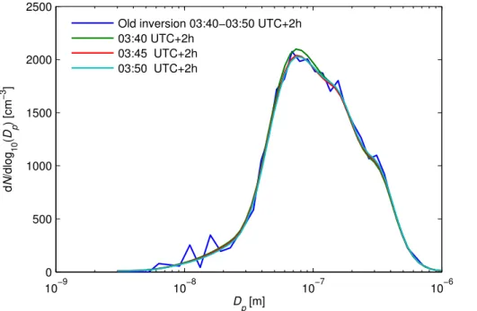
As a first test of the algorithm, let us consider periods without fluctuations, meaning periods for which the old algorithm performed well. As expected, for these periods our results agree well with the results from the old algorithm. The only clear difference is 20

(16)

AMTD

8, 10283–10317, 2015

B. Mølgaard et al.

Title Page

Tables Figures

◭ ◮

Back Close

Full Screen / Esc

Discussion

P

a

per

|

Discussion

P

a

per

|

Discussion

P

a

per

|

Discussion

P

a

per

|

smoother size distributions seem more plausible and were, indeed, obtained using a proper description of the count statistics in the likelihood function as described in Sect. 2.4.1 (the smoothness was also affected by the prior).

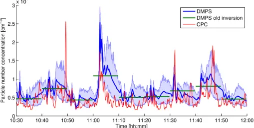
In our next example (2 March 10:30–12:00 UTC+2 h) the evolution of the size distri-bution was as shown in Fig. 6. Clearly, the total particle number concentration fluctu-5

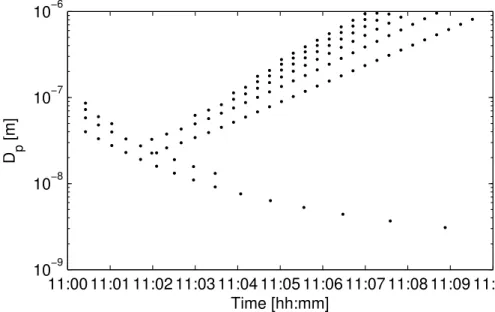
ated a lot and some changes in the size are also seen. At any given time, dN/dlog10Dp changes smoothly as a function of size. The variances in Fig. 7 reflect the distance in time and particle size to the nearest measurements: the further these measurements are, the greater the variance is. In Fig. 4 we showed the training inputs for one scan, and in Fig. 7 low variance areas appear around the training inputs of nine subsequent 10

scans.

The time evolution of the particle number concentrations obtained with the DMPS agrees well with the CPC measurements (Fig. 8), although the CPC generally shows lower concentration. The reason for this difference is that the CPC measurements are not corrected for particle losses in the sampling lines. The peaks generally occur at the 15

same time, although a few of the peaks in the CPC data are not reflected in concentra-tions obtained from the DMPS. For instance, the peak at 10:49 UTC+2 h is only seen in the CPC data. At this time, DMPS-1 measured 3 nm particles, and DMPS-2 measured particles with diameters of more than 500 nm. No clear sign of an elevated concen-tration are seen in these measurements, and thus no inversion algorithm will be able 20

to reproduce this peak. In general, with the set-up of our twin-DMPS, peaks occurring during the last 3–5 min of a scan are often not observed. On the other hand, when both DMPSs measure in the range from 10 to 50 nm, fluctuations in the concentration are most likely observed and our algorithm is able to extract these fluctuating concentra-tions well. For instance, the peak occurring around 11:03 UTC+2 h was well observed 25

(17)

AMTD

8, 10283–10317, 2015

B. Mølgaard et al.

Title Page

Tables Figures

◭ ◮

Back Close

Full Screen / Esc

Discussion

P

a

per

|

Discussion

P

a

per

|

Discussion

P

a

per

|

Discussion

P

a

per

|

size distributions which are much more realistic, but we do not know how close these estimates are to the actual size distributions, because we have no size distribution data from other instruments. In general, the size information during peaks is limited because of the low number of DMPS measurements available.

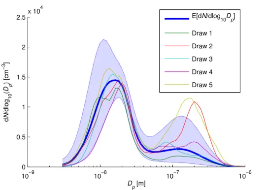
Even less size information is available for the brief concentration peak occurring 5

between 11:31:25 and 11:32:00 UTC+2 h. According to the CPC measurements, the top of the peak occurred at 11:31:50 UTC+2 h which was during the waiting time in both DMPSs, so the peak is not as high according to the DMPS measurements. The few DMPS measurements which were affected by this concentration peak were all for particles in the size range 19 to 23 nm, and these suggested higher dN/dlog10Dp at 10

19 nm than at 23 nm, although this difference could be due to temporal fluctuation. Our algorithm gives the size distribution seen in Fig. 10 at 11:31:45 UTC+2 h and, as expected, dN/dlog10Dp shows a decrease between 19 and 23 nm. The sampled size distributions give examples of what the size distribution may have looked like, and they have maxima between 13 and 20 nm. This seems reasonable given the available 15

size information and the general low values of dN/dlog10Dpat the smallest diameters (Fig. 6). The accumulation mode seen at diameters around 150 nm in Fig. 10 is due to the smoothing in time. Figure 6 shows such a mode for about half an hour around this time. Considering this accumulation mode, our algorithm suggests that its concen-tration fluctuations are simultaneous with the fluctuations at smaller sizes (see Fig. 6). 20

This is caused by the smoothing in size. Fast fluctuations are not observed when the DMPS measures in the accumulation mode, so we do not expect them to occur in the accumulation mode at other times either. The accumulation mode particles have a long life time in the atmosphere and they may originate from distant sources, while the par-ticles smaller than 25 nm most likely originate from nearby traffic emissions (Hussein 25

et al., 2014). However, we used a stationary covariance function with two length scales

(18)

how-AMTD

8, 10283–10317, 2015

B. Mølgaard et al.

Title Page

Tables Figures

◭ ◮

Back Close

Full Screen / Esc

Discussion

P

a

per

|

Discussion

P

a

per

|

Discussion

P

a

per

|

Discussion

P

a

per

|

ever, implementing such a covariance function is not straight-forward. With the current covariance function,ltwill be a compromise between the actual time scales at different sizes. Thus, we expect too much smoothing in the time dimension at small diameters and, as noted above, too little at larger diameters.

To evaluate the performance for the processed 10 day period, we compared mean 5

particle number concentrations obtained from the DMPS and the CPC data at 10 min and 30 s resolution. At 10 min resolution the correlation between the means from the two instruments was 0.984. For comparison, when processing the DMPS data with the old inversion algorithm, the obtained correlation is somewhat lower: 0.967. At the higher time resolution we calculated correlations for each scan separately and Fig. 11 10

shows a histogram of these correlations. Clearly, for most scans there is a good corre-lation and our algorithm extracts information of the time evolution, which was lost with the old algorithm. However, for 11 % of the scans, the correlation is negative, reflecting a disagreement between time evolutions obtained from the DMPS with our algorithm and from the CPC. We have investigated all eight cases for which the correlation is 15

smaller than₋0.75. In two cases the concentration was almost constant according to both instruments, and it seems that small fluctuations caused the negative correlation by chance. In the remaining cases, concentration changes not observed by the DMPS seem to be at least part of the reason. Let us illustrate this with an example (Fig. 12). For the time interval 10:40–10:50 UTC+2 h, the correlation was₋0.87. The CPC mea-20

surements show that the concentration was higher after 10:45 UTC+2 h than before, and at 10:50 UTC+2 h it started decreasing. According to our analysis of the DMPS data, most of the particles had diameters between 7 and 70 nm during this period, but particles in this range were not measured by the DMPS after 10:45 UTC+2 h, so the slightly elevated concentration was not observed. This elevation ended at 10:50 25

(19)

AMTD

8, 10283–10317, 2015

B. Mølgaard et al.

Title Page

Tables Figures

◭ ◮

Back Close

Full Screen / Esc

Discussion

P

a

per

|

Discussion

P

a

per

|

Discussion

P

a

per

|

Discussion

P

a

per

|

to the CPC. However, it seems that our model fits that data well also during this period, meaning that the countsy agree well with the rate parametersλ (data not shown). If we specifically consider the first two minutes of each of the scans in Fig. 12, the CPC showed on average slightly lower concentration during 10:40–10:42 UTC+2 h than dur-ing the other two-minute periods. However, compardur-ing these three periods the DMPS 5

counts were clearly highest during 10:40–10:42 UTC+2 h. This gives some indication that the relatively high concentration in the beginning of this scan is supported by the DMPS data. The negative correlation during this scan seems to originate from the mea-surements rather than from any problem in our inversion algorithm. In our investigation of other scans with negative correlations did not suggest problems with the inversion 10

either. So despite these occasional negative correlations, it seems that our model ex-tracts the information of the concentration time evolution well from the available DMPS measurements.

The results above are based on a few simplifying assumptions. We assumed that the particle concentration only changes a little during each measurement. This is not 15

necessarily always the case, but the approximation in Eq. (3) is correct at least at some point during the measurement. For DMPS-2 most of the measurements are short (∼5 s) and any error arising from this approximation can be considered as a minor er-ror in the timing. For DMPS-1, each measurement at the smallest sizes last around a minute, but strong fluctuations are rare at these sizes. In principle, we could have 20

split the time intervals into smaller pieces, and summed up their contribution, but the minor improvement would not have justified the extra computational cost. We ignored particles larger than 1 µm, but with the chosen data this seems to be a minor issue. We also ignored the uncertainties of sample and sheath flows, so our uncertainties are somewhat underestimated. The sample flows affect the likelihood directly through 25

(20)

AMTD

8, 10283–10317, 2015

B. Mølgaard et al.

Title Page

Tables Figures

◭ ◮

Back Close

Full Screen / Esc

Discussion

P

a

per

|

Discussion

P

a

per

|

Discussion

P

a

per

|

Discussion

P

a

per

|

In summary, our algorithm extracts well the time evolution of the particle number concentration from the available DMPS data, and in absence of fluctuations the ob-tained size distributions fit well with results from the old algorithm. During fluctuations, only little information about the particle sizes is available, and the uncertainties of the size distributions are considerable. Due to lack of independent size distribution data, 5

a quantitative evaluation of the size distributions obtained for periods with fluctuation was impossible, but there is no doubt that these size distributions are much closer to the truth than the ones obtained with the old algorithm.

In principle, this method should work for the SMPS as well, but we expect the imple-mentation to be more difficult. The continuous scan needs to be divided into a number 10

of counting intervals. If the counting intervals are long, the peaks of the transfer function will be much wider. On the other hand, if the counting intervals are short, the number of training inputs in our model will be high, and our algorithm will be much slower.

4 Conclusions

We have developed a new algorithm (provided in the Supplement) based on a Gaus-15

sian Process model for processing DMPS data, and we tested it with data from a twin-DMPS in a suburban location. Our algorithm derives dN/dlog10Dpas a function ofDp andt based on DMPS measurements and smoothness assumptions. Because these assumptions are more realistic than the assumption of a stationary aerosol, also the derived size distributions are much more realistic. We compared particle number con-20

centrations with independent CPC measurements, and found a good agreement. The higher accuracy of the particle number size distributions can benefit studies of aerosols in urban locations and other places with fluctuating size distributions. The higher time resolution is useful, for instance, when attempting to pinpoint sources, given that other data, such as wind observations, exists at a good time resolution. Particle 25

(21)

instru-AMTD

8, 10283–10317, 2015

B. Mølgaard et al.

Title Page

Tables Figures

◭ ◮

Back Close

Full Screen / Esc

Discussion

P

a

per

|

Discussion

P

a

per

|

Discussion

P

a

per

|

Discussion

P

a

per

|

ments as well, but this algorithm offers an improvement both for existing and future DMPS data without any need to purchase new hardware.

The Supplement related to this article is available online at doi:10.5194/amtd-8-10283-2015-supplement.

Acknowledgements. J. Vanhatalo and N. L. Prisle were funded by the Academy of Finland

5

(grants 266349 and 257411, respectively).

References

Gelfand, A. E., Diggle, P. J., Fuentes, M., and Guttorp, P.: Handbook of Spatial Statistics, CRC Press, Boca Raton, FL, USA, 2010. 10289

Gelman, A.: Prior distributions for variance parameters in hierarchical models, Bayesian

Anal-10

ysis, 1, 515–533, doi:10.1214/06-BA117A, 2006. 10291

Gelman, A., Carlin, J. B., Stern, H. S., Dunson, D. B., Vehtari, A., and Rubin, D. B.: Bayesian Data Analysis, 3rd edn., Chapman and Hall/CRC, Boca Raton, FL, USA, 2013. 10294 Hinds, W. C.: Aerosol Technology: Properties, Behavior, and Measurement of Airborne

Parti-cles, John Wiley and Sons, Inc., Hoboken, NJ, USA, 1999. 10287

15

Hussein, T., Mølgaard, B., Hannuniemi, H., Martikainen, J., Järvi, L., Wegner, T., Ripamonti, G., Weber, S., Vesala, T., and Hämeri, K.: Fingerprints of the urban particle number size dis-tribution in Helsinki, Finland: local versus regional characteristics, Boreal Environ. Res., 19, 1–20, 2014. 10299

Järvi, L., Hannuniemi, H., Hussein, T., Junninen, H., Aalto, P. P., Hillamo, R., Mäkelä, T.,

Kero-20

nen, P., Siivola, E., Vesala, T., and Kulmala, M.: The urban measurement station SMEAR III: Continuous monitoring of air pollution and surface-atmosphere interactions in Helsinki, Finland, Boreal Environ. Res., 14 (Supplement A), 86–109, 2009. 10285, 10292

Mamakos, A., Ntziachristos, L., and Samaras, Z.: Diffusion broadening of DMA trans-fer functions. Numerical validation of Stolzenburg model, J. Aerosol Sci., 38, 747–763,

25

(22)

AMTD

8, 10283–10317, 2015

B. Mølgaard et al.

Title Page

Tables Figures

◭ ◮

Back Close

Full Screen / Esc

Discussion

P

a

per

|

Discussion

P

a

per

|

Discussion

P

a

per

|

Discussion

P

a

per

|

Maricq, M. M.: Bipolar diffusion charging of soot aggregates, Aerosol Sci. Tech., 42, 247–254, doi:10.1080/02786820801958775, 2008. 10301

O’Hagan, A.: Curve fitting and optimal design for prediction, J. Roy. Stat. Soc. B Met., 40, 1–42, 1978. 10288

Rasmussen, C. E. and Williams, C. K. I.: Gaussian Processes for Machine Learning, The MIT

5

Press, Cambridge, MA, USA, available at: www.gaussianprocess.org/gpml (last access: 1 October 2015), 2006. 10286, 10288, 10289, 10291, 10294, 10295, 10296

Rue, H., Martino, S., and Chopin, N.: Approximate Bayesian inference for latent Gaussian models by using integrated nested Laplace approximations, J. Roy. Stat. Soc. B, 71, 1–35, doi:10.1111/j.1467-9868.2008.00700.x, 2009. 10297

10

Stolzenburg, M. R.: An ultrafine aerosol size distribution measuring system, PhD thesis, De-partment of Mechanical Engineering, University of Minnesota, USA, 1988. 10288

Tierney, L. and Kadane, J. B.: Accurate approximations for posterior moments and marginal densities, J. Am. Stat. Assoc., 81, 82–86, 1986. 10297

Vanhatalo, J.: Speeding Up the Inference in Gaussian Process Models, PhD thesis, School of

15

Science and Technology, Aalto University, Finland, 2010. 10296, 10297

Vanhatalo, J., Pietiläinen, V., and Vehtari, A.: Approximate inference for disease mapping with sparse Gaussian processes, Stat. Med., 29, 1580–1607, doi:10.1002/sim.3895, 2010. 10289, 10294, 10296, 10297

Vanhatalo, J., Riihimäki, J. P., Hartikainen, J., Jylänki, P., Tolvanen, V., and Vehtari, A.: GPstuff:

20

Bayesian Modeling with Gaussian Processes, J. Mach. Learn. Res., 14, 1175–1179, 2013. 10294, 10296, 10297

Voutilainen, A. and Kaipio, J. P.: Estimation of non-stationary aerosol size distributions using the state-space approach, J. Aerosol Sci., 32, 631–648, doi:10.1016/S0021-8502(00)00110-5, 2001. 10286

25

Voutilainen, A. and Kaipio, J. P.: Estimation of time-varying aerosol size distributions – exploita-tion of modal aerosol dynamical models, J. Aerosol Sci., 33, 1181–1200, doi:10.1016/S0021-8502(02)00062-9, 2002. 10286

Voutilainen, A. and Kaipio, R.: Sequential Monte Carlo estimation of aerosol size distributions, Comput. Stat. Data An., 48, 887–908, doi:10.1016/j.csda.2004.03.011, 2005. 10286

30

(23)

AMTD

8, 10283–10317, 2015

B. Mølgaard et al.

Title Page

Tables Figures

◭ ◮

Back Close

Full Screen / Esc

Discussion

P

a

per

|

Discussion

P

a

per

|

Discussion

P

a

per

|

Discussion

P

a

per

|

Hüglin, C., Fierz-Schmidhauser, R., Gysel, M., Weingartner, E., Riccobono, F., Santos, S., Grüning, C., Faloon, K., Beddows, D., Harrison, R., Monahan, C., Jennings, S. G., O’Dowd, C. D., Marinoni, A., Horn, H.-G., Keck, L., Jiang, J., Scheckman, J., McMurry, P. H., Deng, Z., Zhao, C. S., Moerman, M., Henzing, B., de Leeuw, G., Löschau, G., and Bastian, S.: Mobility particle size spectrometers: harmonization of technical standards and data structure to

fa-5

(24)

AMTD

8, 10283–10317, 2015

B. Mølgaard et al.

Title Page

Tables Figures

◭ ◮

Back Close

Full Screen / Esc

Discussion

P

a

per

|

Discussion

P

a

per

|

Discussion

P

a

per

|

Discussion

P

a

per

|

Figure 1.Size distributions from 2 March 2015 according to the old inversion algorithm, which

(25)

AMTD

8, 10283–10317, 2015

B. Mølgaard et al.

Title Page

Tables Figures

◭ ◮

Back Close

Full Screen / Esc

Discussion

P

a

per

|

Discussion

P

a

per

|

Discussion

P

a

per

|

Discussion

P

a

per

|

10−9 10−8 10−7 10−6

0 0.5 1 1.5 2 2.5

3x 10

4

d

N

/dlog

10

(

D p

) [cm

−3

]

D_p [m]

10:50−11:00 UTC+2h 11:00−11:10 UTC+2h 11:10−11:20 UTC+2h

Figure 2. Three particle number size distributions from 2 March 2015 according to the old

(26)

AMTD

8, 10283–10317, 2015

B. Mølgaard et al.

Title Page

Tables Figures

◭ ◮

Back Close

Full Screen / Esc

Discussion

P

a

per

|

Discussion

P

a

per

|

Discussion

P

a

per

|

Discussion

P

a

per

|

SMEAR III

University

Campus

Vegetated

area

100 m Major road

Minor road

(27)

AMTD

8, 10283–10317, 2015

B. Mølgaard et al.

Title Page

Tables Figures

◭ ◮

Back Close

Full Screen / Esc

Discussion

P

a

per

|

Discussion

P

a

per

|

Discussion

P

a

per

|

Discussion

P

a

per

|

11:00 11:01 11:02 11:03 11:04 11:05 11:06 11:07 11:08 11:09 11:10

10−9

10−8

10−7

10−6

Time [hh:mm]

D p

[m]

Figure 4. Training inputs for the scan on 2 March between 11:00 and 11:10 UTC+2 h. For

(28)

AMTD

8, 10283–10317, 2015

B. Mølgaard et al.

Title Page

Tables Figures

◭ ◮

Back Close

Full Screen / Esc

Discussion

P

a

per

|

Discussion

P

a

per

|

Discussion

P

a

per

|

Discussion

P

a

per

|

10−9 10−8 10−7 10−6

0 500 1000 1500 2000 2500

d

N

/dlog

10

(

D p

) [cm

−3

]

D

p [m]

Old inversion 03:40−03:50 UTC+2h 03:40 UTC+2h

03:45 UTC+2h 03:50 UTC+2h

Figure 5. The size distribution obtained with the old inversion algorithm and expected size

(29)

AMTD

8, 10283–10317, 2015

B. Mølgaard et al.

Title Page

Tables Figures

◭ ◮

Back Close

Full Screen / Esc

Discussion

P

a

per

|

Discussion

P

a

per

|

Discussion

P

a

per

|

Discussion

P

a

per

|

Figure 6.Expected size distributions on 2 March between 10:30 and 12:00 UTC+2 h. The ticks

(30)

AMTD

8, 10283–10317, 2015

B. Mølgaard et al.

Title Page

Tables Figures

◭ ◮

Back Close

Full Screen / Esc

Discussion

P

a

per

|

Discussion

P

a

per

|

Discussion

P

a

per

|

Discussion

P

a

per

|

Figure 7.Posterior variance off on 2 March between 10:30 and 12:00 UTC+2 h. The ticks on

(31)

AMTD

8, 10283–10317, 2015

B. Mølgaard et al.

Title Page

Tables Figures

◭ ◮

Back Close

Full Screen / Esc

Discussion

P

a

per

|

Discussion

P

a

per

|

Discussion

P

a

per

|

Discussion

P

a

per

|

10:300 10:40 10:50 11:00 11:10 11:20 11:30 11:40 11:50 12:00 0.5

1 1.5 2 2.5

3x 10

4

Time [hh:mm]

Particle number concentration [cm

−3]

DMPS

DMPS old inversion CPC

(32)

AMTD

8, 10283–10317, 2015

B. Mølgaard et al.

Title Page

Tables Figures

◭ ◮

Back Close

Full Screen / Esc

Discussion

P

a

per

|

Discussion

P

a

per

|

Discussion

P

a

per

|

Discussion

P

a

per

|

10−9 10−8 10−7 10−6

0 0.5 1 1.5 2 2.5

3 x 10

4

d

N

/dlog

10

(

D p

) [cm

−3

]

D_p [m] Old inversion 11:00 − 11:10 11:00:35

11:02:35 11:04:35 11:06:35

Figure 9. Expected size distribution before, during, and after the peak on 2 March at

(33)

AMTD

8, 10283–10317, 2015

B. Mølgaard et al.

Title Page

Tables Figures

◭ ◮

Back Close

Full Screen / Esc

Discussion

P

a

per

|

Discussion

P

a

per

|

Discussion

P

a

per

|

Discussion

P

a

per

|

10−9 10−8 10−7 10−6

0 0.5 1 1.5 2 2.5x 10

4

d

N

/dlog

10

(

D p

) [cm

−3

]

D_p [m]

E[dN/dlog

10Dp]

Draw 1

Draw 2

Draw 3

Draw 4

Draw 5

Figure 10.Expected size distribution with 95 % posterior intervals and five size distributions

(34)

AMTD

8, 10283–10317, 2015

B. Mølgaard et al.

Title Page

Tables Figures

◭ ◮

Back Close

Full Screen / Esc

Discussion

P

a

per

|

Discussion

P

a

per

|

Discussion

P

a

per

|

Discussion

P

a

per

|

−1 −0.5 0 0.5 1

0 50 100 150 200 250

Correlation

Number of scans

Figure 11.Histogram of correlations between 30 s mean particle number concentrations

(35)

AMTD

8, 10283–10317, 2015

B. Mølgaard et al.

Title Page

Tables Figures

◭ ◮

Back Close

Full Screen / Esc

Discussion

P

a

per

|

Discussion

P

a

per

|

Discussion

P

a

per

|

Discussion

P

a

per

|

10:300 10:35 10:40 10:45 10:50 10:55 11:00 200

400 600 800 1000 1200 1400 1600 1800

Time [hh:mm]

DMPS

DMPS old inversion CPC