Abstract— This paper presents a performance comparison between
known propagation Models through least squares tuning algorithm for 5.8 GHz frequency band. The studied environment is based on the 12 cities located in Amazon Region. After adjustments and simulations, SUI Model showed the smaller RMS error and standard deviation when compared with COST231-Hata and ECC-33 models.
Index Terms— 5.8 GHz band, Amazon Region, Linear Least Squares, Propagation models.
I. INTRODUCTION
Since the constant increase of the wireless networks, studies of signal propagation are needed to
ensure an efficient Pre-Project Stage in coverage and quality of services. This paper presents a study
of the signal propagation in 5.8 GHz on Amazon region cities.
A performance comparison between known propagation models is made for an Amazon Region
environment. The least squares tuning algorithm has been used to adjust the models to the
measurements. It is important to remember that the terms related to reception and transmission heights
in the models equations have been left unchanged. Although the models adjustments, differences in
how the models work with reception and transmission height have influence in RMS error and
standard deviation which are the metrics adopted in this work.
This paper is organized as follows. In section II is presented explanations about the environment
and the data acquisition. In section III a description of the propagation models is made. In section IV
the least squares tuning algorithm is presented. In section V simulations and results are shown and
finally, section VI shows the conclusions.
II. ENVIRONMENT AND DATA ACQUISITION
The collected data have been carried out in 12 cities on Pará State at Amazon Region, Brazil. These
cities are known by their woodland environments. The vegetation normally appears mixed with the
residential and commercial constructions resulting in a single medium. An example of Amazon region
Comparison Between Known Propagation
Models Using Least Squares Tuning
Algorithm on 5.8 GHz in Amazon Region
Cities
Bruno S. L. Castro, Márcio R. Pinheiro, Gervásio P. S. Cavalcante
Federal University of Pará (UFPA), Augusto Correa Avenue S/N, ZIPCODE: 66075-900, Belém-Pará-Brazil, e-mails:[email protected],[email protected] and [email protected]
Igor R. Gomes, Oziel de O. Carneiro
city is shown in Fig.1.
Fig. 1. Aerial view of Santarém city in Pará State, Brazil
Different of the traditional measuring campaigns [1]-[2] that are made with continuous data
collection in a mobile unit, this data acquisition has been carried out by taking the punctual RSSI
(Received Signal Strength Indicator) in 335 fixed clients installed in 12 cities that have been
contemplated with the Digital Inclusion Pará State Government Project named NavegaPará [3]. The
project consists of WLL (Wireless Local Loop) networks installed in the cities, bringing broadband
access and multimedia services. It is interesting to analyze this collected data because fixed clients
have different distances with respect to their Base Stations and different installation heights. From the
collected RSSI it can be found the path loss for each client by using values of transmission power,
transmission gain and reception gain.
The process for obtaining the distances between the clients and base stations is based on the
coordinates that was collected during the implantation stage of these networks.
III. PROPAGATION MODELS
The propagation models used in this paper are COST231-Hata, SUI Model and ECC-33 model
whose have reference in some performance comparison works [4]-[5]-[6].
A. Stanford University Interim (SUI) Model
SUI Model has had in your development the Stanford University participation. Variables involved
in model prediction process are adopted for frequencies below 11 GHz. It is interesting to evaluate
model performance for this case because SUI Model employs terrain properties on its equations so the
base for calculating the propagation loss can be accomplished in an non-ideal way different of the free
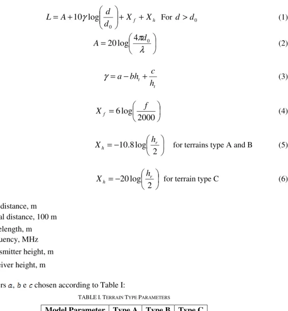
The base of the propagation model and the environment characterization are represented by the
following equations [7]:
h f
X
X
d
d
A
L
+
+
+
=
0log
10
γ
For d >d0 (1) =
λ
π
0 4 log 20 dA (2)
t t
h c bh a− + =
γ
(3) = 2000 log 6 f
Xf (4)
− = 2 log 8 . 10 r h h
X for terrains type A and B (5)
− = 2 log 20 r h h
X for terrain type C (6)
Where:
d- Link distance, m
0
d - Initial distance, 100 m
λ
- Wavelength, mf
- Frequency, MHzt
h - Transmitter height, m
r
h
- Receiver height, mParameters , e chosen according to Table I:
TABLEI.TERRAIN TYPE PARAMETERS
Model Parameter Type A Type B Type C
a 4.6 4 3.6
b 0.0075 0.0065 0.005
c 12.6 17.1 20
Table I is based on terrain types defined in [7].
B. COST 231 - Hata
This one is an extension of Okumura-Hata Model. It was made to embrace a frequency range from 1500 MHz to 2000 MHz. The propagation loss obtained can be calculated through the following equation:
( )
f( )
hte a( )
hre(
( )
hte)
( )
d cmL=46.3+39.9log −13.82log − + 44.9−6.55log log + (7)
( )
h =(
1.1log( )
f −0.7)
h −(
1.56f −0.8)
a re re for small and medium cities (8)
( )
h
re=
3
.
2
(
log
(
11
.
75
h
re)
)
2−
4
.
97
Where:
f
- Frequency, MHzd- Link distance, m
te
h - Transmitter height, m
re
h - Receiver height, m
m
c - 0 dB for soft and suburban areas and 3 dB for dense urban areas
C. ECC-33Model
ECC-33 is a model from Electronic Communication Committee based on analysis in 3.4 and 3.8 GHz band. The path loss is obtained from de following equations [4]:
r b bm
fs A G G A
L= + − − (10)
( )
d( )
fAfs =92.4+20log +20log (11)
( )
( )
(
( )
)
2log
56
.
9
log
894
.
7
log
83
.
9
41
.
20
d
f
f
A
bm=
+
+
+
(12)( )
(
)
2log 8 . 5 958 . 13 200
log h d
G b
b +
= (13)
And for medium city environments,
( )
(
42
.
57
+
13
.
7
log
)
(
log
( )
−
0
.
585
)
=
rr
f
h
G
(14)Where:
d- Link distance, m
f
- Frequency, GHzb
h - Transmitter height, m
r
h
- Receiver height, mIV. LEAST SQUARES ALGORITHM
Due to the different characteristics of the environment where the models have been made, a tuning
proceeding is needed to adjust model parameters to the measured data.
Least Squares (LS) criterion is useful for linear adjustment cases. In this situation, the algorithm is
represented by the idea of minimizing the sum of the squares of the differences between measured
data and predicted data. These differences become an error function expressed as follows:
(
)
2 1∑
=−
=
n i i iL
Y
E
(15)Where:
- Error function
- Number of total used data
- Measured data
The distance and frequency terms in the models equations were adjusted by the algorithm, however,
the transmission and reception heights terms were not included in least squares tuning.
More details about LS algorithm applied in tuning method are described in [1]-[2].
V. SIMULATIONS AND RESULTS
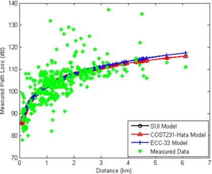
Simulations have been done considering the mean and specific installation heights of the clients
located at the 12 cities in study. The data obtained in the simulations are shown in Fig. 2-5.
Fig. 2. Propagation models performance using mean reception heights of the clients
After simulations, the obtained values of RMS error (dB) and standard deviation (dB) for all three
models are shown in the Table II, before and after tuning.
TABLEII.RESULTS FOR MEAN INSTALLATION HEIGHT
Models RMS Error Before
Standard Deviation
Before
RMS Error After
Standard Deviation After
SUI 14.66 6.60 6.25 4.47
COST231-Hata 11.29 5.54 6.25 4.47
ECC-33 28.03 7.64 6.24 4.43
Fig. 4. Propagation models performance using specific reception heights of the clients
For the specific client heights, the obtained results are shown in the Table III, for the RMS error and
standard deviation as well.
TABLEIII.RESULTS FOR SPECIFIC INSTALLATION HEIGHT
Models RMS
Error (Before)
Standard Deviation (Before)
RMS Error After
Standard Deviation After
SUI 15.26 6.88 7.22 4.84
COST231-Hata 17.27 9.88 15.51 10.97
ECC-33 31.32 10.67 11.12 6.99
From the results in Table II, it is seem that SUI, COST231-Hata and ECC-33 models, reach the
same RMS error (6.2 dB) when mean reception height is used in least squares tuning.
In the other hand, when specific client installation height was used for tuning process, SUI Model
obtained the best improvement with a RMS error of 7.22 dB and COST 231-Hata had the worst one
equal to 15.51 dB. RMS errors have obtained a maximum improvement about 20 dB (ECC-33 Model)
and a minimum improvement around 2 dB (COST231-Hata Model). The minor standard deviation
value belongs to SUI Model.
Results are relevant because RSSI collecting process has been performed in peculiar site-specific
clients. Variations in models predictions, from Fig. 4 and Fig. 5, are justified because each client has a
specific CPE (customer premises equipment) installation height.
RMS error (RE) and standard deviation (SD) values for all 12 cities in study are shown in Table IV.
TABLEIV.RESULTS FOR SPECIFIC INSTALLATION HEIGHT
Cities SUI Model COST231-Hata Model ECC-33 Model
RE SD RE SD RE SD
Abaetetuba 7.05 4.24 27.14 10.31 10.95 6.45
Altamira 5.81 3.93 20.26 9.64 10.61 7.61
Barcarena 10.64 6.71 33.48 14.63 11.91 6.86
Itaituba 7.34 4.89 30.26 10.14 10.24 6.42
Jacundá 5.21 3.04 35.27 10.30 7.11 4.02
Marabá 7.14 4.80 26.25 17.77 14.67 9.04
Pacajá 5.25 2.69 33.95 7.62 9.11 5.02
Rurópolis 4.50 2.78 30.45 8.59 7.44 4.70
Santarém 8.86 6.21 22.88 13.18 13.37 7.80
Tailândia 8.08 4.96 37.05 11.22 10.36 6.51
Tucurí 7.87 6.33 24.65 10.70 11.42 7.62
VI. CONCLUSION
In this paper, a performance comparison between COST231-Hata, Stanford University Interim
(SUI) and ECC-33 models is made for an Amazon Region environment. At the final performance
evaluation, SUI Model has shown a better behavior than COST231-Hata and ECC-33 Models. Based
on the obtained results, a proposal for future works can consider an adjustment of SUI Model by
changing some parameters or adding a term which is related to some new environment feature. It is
also foreseen an adjustment in SUI model for path loss prediction in mobility conditions. For such a
purpose, measurement campaigns will be carried out.
ACKNOWLEDGMENT
Authors would like to thank the Pará State Data Processing Company (PRODEPA) for accessing
important information to the work development.
This work was supported by CNPq under covenant 573939/2008-0(INCT-CSF) and FAPESPA /
UFPA / FADESP/SEDECT, Nº. 067/2008.
REFERENCES
[1] M. Yang, W. Shi, “Linear Least Square Method of Propagation Model Tuning for 3G Radio Network Planning”, Fourth International Conference on Natural Computation ICNC, Jinan, 18-20 October 2008, pp. 150-154.
[2] G. R. Pallardó, “On DVB-H Radio Frequency Planning: Adjustment of a Propagation Model Through Measurement Campaign Results”, Master’s Thesis, Department of technology and Built Enviroment, University of Gävle, Sweden, 2008.
[3] NavegaPará Project. Available in: http://www.navegapara.pa.gov.br/
[4] V. S. Abhayawardhana, I.J. Wassell, D. Crosby, M.P. Sellars and M.G. Brown, “Comparison of Empirical Propagation Path Loss Models for Fixed Wireless Access Systems”, IEEE 61st Vehicular Technology Conference VTC, Stockholm, 30 May-1 June 2005, pp. 73-77.
[5] J. Milanovic, S. Rimac-Drje, K. Bejuk, “Comparison of Propagation Models Accuracy for Wimax on 3.5 GHz”, 14th IEEE International Conference on Circuits and Systems ICECS, Marrakech, 11-14 December 2007, pp. 111-114.
[6] T. Schwengler, M. Gilbert, “Propagation Models at 5.8 GHz - Path Loss & Building Penetration”, IEEE Radio and Wireless Conference RAWCON, Denver, 10-13 December 2000, pp. 119-124.