Abstract
The thermo-hydro-mechanical problems associated with a poroelas-tic half-space soil medium with variable properties under general-ized thermoelasticity theory were investigated in this study. By remaining faithful to Biot’s theory of dynamic poroelasticity, we idealized the foundation material as a uniform, fully saturated, poroelastic half-space medium. We first subjected this medium to time harmonic loads consisting of normal or thermal loads, then investigated the differences between the coupled thermohydro-mechanical dynamic models and the thermo-elastic dynamic mod-els. We used normal mode analysis to solve the resulting non-dimensional coupled equations, then investigated the effects that non-dimensional vertical displacement, excess pore water pressure, vertical stress, and temperature distribution exerted on the poroe-lastic half-space medium and represented them graphically.
Keywords
Coupled thermo-hydro-mechanical dynamic, Generalized thermoelasticity, Thermo-elastic dynamic, Poroelastic, Normal mode analysis
Normal Mode Analysis to a Poroelastic Half-Space
Problem under Generalized Thermoelasticity
NOMENCLATURE
w
c Heat capacity of pore water
s
c Heat capacity of solid grains e Volumetric strain of soil
g Gravity
K Coefficient of thermal conductivity
d
k Coefficient of permeability
m Volumetric heat capacity of medium
Chunbao Xiong a, 1 Ying Guo a, 2 Yu Diao a, 3 *
a School of Civil Engineering, Tianjin
University. Weijin Road 92, Nankai District, Tianjin. P.R. China
1 Email: [email protected] 2 Email: [email protected] 3 Email: [email protected]
* Corresponding author
http://dx.doi.org/10.1590/1679-78253611
NOMENCLATURE (continuation)
0
n Porosity
p Excess pore water pressure
Q Magnitude of applied temperature q Magnitude of applied load
T Absolute temperature of medium
0
T Reference temperature
s
Thermal expansion coefficient of solid grains
w
Thermal expansion coefficient of pore water
1
3 2
s G
ij
Components of strain tensor
T T0 ,G
Lame’s constants
Poisson ratio Density of medium
w
Density of pore water
s
Density of solid grains
ij
Components of stress tensor
Thermal relaxation time
1 INTRODUCTION
The effects of temperature on the behavior of soil is an important engineering concern. Temperature can impact the disposal of high-level radioactive waste, the extraction of oil or geothermal energy, the storage of hot fluids, road subgrades, and furnace foundations. The theory of thermoelasticity was developed in order to analyze these problems associated with thermodynamics.
A great deal of research attention has been focused on the wave propagation problem in context of generalized thermoelasticity. Singh (2007) solved a two-dimensional homogeneous, isotropic gen-eralized thermoelastic half-space problem in the context of Lord and Shulman theory of gengen-eralized thermoelasticity. The propagation of waves in a transversely isotropic micropolar medium pos-sessing thermoelastic properties under three different theories are discussed by Kumar and Gupta (2010). Bijarnia and Singh (2012) investigated the propagation of four different plane waves in a solid half-space with diffusion in the context of the Lord and Shulman theory of generalized thermo-elasticity. Lotfy (2014) investigated a two-temperature problem for an isotropic homogeneous elastic half-space under three thermoelastic theories. Lotfy and Hassan (2014) solved a thermoelastic wave propagation problem for a half-space media subject to thermal shock based on the two-temperature theory of thermoelasticity. Abo-Dahab et al. (2015) studied the effects of magnetic field, relaxation times, and rotation on the propagation of surface waves in the context of Green-Lindsay theory. Singh (2016) explored plane wave propagation in a solid half-space which is rotating, transversely isotropic, two-temperature thermoelastic without energy dissipation. Lotfy (2016) introduced the dual-phase-lag (DPL) heat transfer model to solve the problem for a isotropic generalized thermoe-lastic medium with an internal heat source.
Wave propagation in a thermoelastic porous media is useful in various engineering fields such as petroleum engineering, chemical engineering, pavement engineering, and nuclear waste management, making it a popular research subject as well. Kumar and Devi (2008) investigated a porous, general-ized thermoelastic medium subjected to thermomechanical boundary conditions permeated with various heat sources. Sherief and Hussein (2012) developed a set of governing equations that effec-tually create a mathematical model of generalized thermoelasticity in poroelastic materials, then, they used this model to solve a thermal shock problem regarding the use of half-space. Abbas and Youssef (2015) solved a two-dimensional problem of a porous material in the context of the frac-tional order generalized thermoelasticity theory with one relaxation time. Wei et al. (2016) studied the reflection and refraction phenomenon that occurs in an oblique incidence longitudinal wave at a plane interface between an isotropic, homogeneous, thermoelastic medium and a porous thermoelas-tic medium. Schanz (2009) provided an overview of several poroelastodynamic models and analyti-cal solutions, and also discussed two different numerianalyti-cal methodologies including the finite element method and the boundary element method.
The role that fluid flow plays in thermoelasticity was neglected in the above studies. With this in mind, we conducted the present study because we believe that a thorough knowledge of hydro-thermal, hydromechanical, and thermal-mechanical processes, as well as knowledge of the interde-pendence of these processes, is necessary to accurately model the coupled behavior of fluid-saturated media. The thermo-hydro-mechanical (THM) coupled behavior of unsaturated soil is a very com-mon physical phenomenon in nature and very worthy of further research.
po-rous space subjected to exponential decaying thermal loading, and derived the thermal consolidation of layered, saturated porous half-space to various thermal loads with time. Bai (2006b) established coupled governing equations for one-dimensional thermal consolidation problems regarding saturat-ed porous msaturat-edia subjectsaturat-ed to cyclical thermal loading. Bassaturat-ed on the thermodynamics of irreversible processes; Bai and Li (2009) investigated a saturated medium with a long cylindrical cavity subject-ed to variable thermal loading and variable hydrostatic pressure. Lu et al. (2010) investigatsubject-ed a porous elastic medium subjected to a normal force and a thermal source in the context of general-ized thermoelastic theory with one relaxation time. Liu et al. (2009; 2010a) developed a method to overcome one-dimensional problems for an isotropic saturated poroelastic medium including a cylin-drical cavity and spherical cavity subjected to a time-dependent thermal/mechanical shock in the context of thermodynamics theory. That same year, Liu et al. (2010b) solved a thermo-hydro-elastodynamic problem in a two-phase porous thermoelastic medium. Bai and Li (2013) developed a spherical space with a spherical cavity based on the irreversible governing equations of saturated porous thermoelastic media and subjected it to variable mechanical and thermal loads. Kumar et al. (2014) investigated the propagation of Lamb waves in solids with layers or half-spaces of inviscid liquid subjected to stress-free boundary conditions in the context of the Green and Lindsay theory of generalized thermoelasticity. Ailawalia and Singla (2016) solved an infinite homogeneous isotropic generalized thermoelastic problem under the Lord and Shulman theory of generalized thermoelastic-ity.
To date, there have been very few works devoted to investigating thermo-hydro-mechanical problems involving normal or thermal loads via normal mode analysis. In this study, we investigat-ed these thermo-hydro-mechanical problems and the characteristic variable properties in a poroelas-tic half-space soil medium in the context of generalized thermoelasporoelas-tic theory. We subjected this poroelastic half-space to time harmonic loads comprised of normal or thermal loads. The foundation material, under Biot’s dynamic poroelastic theory, was idealized as a uniform, fully saturated poroe-lastic half-space. The distributions of non-dimensional vertical displacement, excess pore water pres-sure, vertical stress, and temperature distribution were obtained by means of normal mode analysis. The numerical results were obtained by performing numerical inversion of the transform integrals. These results were then used to analyze the differences between the two methods of coupled ther-mo-hydro-mechanical dynamic model (THMD) and thermoelastic dynamic model (TMD).
2 BASIC EQUATIONS
We consider the problem of a saturated, homogenous, isotropic porous elastic half-space. Based on theory of three-dimensional consolidation which proposed by Biot (1941), we assume that solid grains are incompressible because the Biot’s effective stress coefficient 1. The dynamic equation for the motion of thermo-hydromechanical coupling in the absence of body forces can be written by Smith and Booker, Bai and Abousleiman, and Bai as follows (1993, 1997, 2006c):
1, , , ,
i jj j ij i i i
Gu G u p u (1)
The equation associated with heat conduction for poroelastic soil can be written by Sherief and Saleh, and Ram et al. as follows (2005, 2008):
2 2
1 0
2 2 ,ii
m T e K
t t t t
(2)
where mn0w wc
1 n0
s sc .Based on Darcy’s law, the equation of mass conservation of water is:
2
2 , 0
w w ii
e e
b p
t t t
(3)
where w d
g
b
.
In the absence of a body force or inner heat source, the constitutive governing equation of thermo-hydromechanical can be written by Smith and Booker as follows (1993):
1
2
ij G ij e p ij
(4)
The strain-displacement relation equation is:
1 , , 2
ij ui j uj i
(5)
3 FORMULATION OF THE PROBLEM
We consider the problem of a saturated, homogenous, isotropic porous elastic half-space soil medi-um subjected to both normal force and thermal loading. The governing equations are written in the context of the Lord and Shulman model, where the body is under no anybody force. The Cartesian coordinate system
x y z, ,
and displacement components ui
u,0,w
are introduced below.These displacement components have the following forms:
, , ,
0,
, ,
x y z
u u x z t u u w x z t (6)
Based on Eqs. (5) and (6), the strain components have the following forms:
1
, , , 0
2
xx zz xz xy yy yz
u w u w
e e e e e e
x z z x
(7)
where e is the cubical dilatation, which is expressed as follows:
u w
e
x z
(8)
22
1 2
e p u
G u G
x x x t
(9)
22
1 2
e p w
G w G
z z z t
(10)
1
2
xx
u
G e p
x
(11)
1
2
zz
w
G e p
z (12) xz u w G z x
(13)
where 2 2 2 2 2 x z
is a two-dimensional Laplace operator.
In order to facilitate the equation, the following non-dimensional quantities are also introduced:
2 2
1
2 2
ij ij
x V x z V z u V u w V w t V t V
p p
G G G
(14)
where m V 2G
K
.
In terms of the non-dimensional quantities in Eq. (14), we can transform Eqs. (2), (3), (9), and (10) into the following forms (dropping primes for convenience):
22 2 2 2
2
1 e p u
u
x x x t
(15)
22 2 2 2
2
1 e p w
w
z z z t
(16)
2 2 0 2 e t t (17)
2 2
1 2 3 2
e e
p
t t t
(18)
Accordingly, the constitutive non-dimensional equations are:
2 2 xx u e p x G (19)
2 2 zz w e p z G xz
u w
z x
(21)
where
2
2 0 1
0 1 2 3
1
2
2 2 w w
T b b G
m G G G
Differentiating Eq. (15) with respect to x, and Eq. (16) with respect to z, then adding them
together, we arrive at follows:
2
2 2 2
2 e p 0
t
(22)
4 NORMAL MODE ANALYSIS
The solutions for the variables that we considered can be decomposed in terms of normal modes in the following form:
, , , ,ij , , , , , ij , exp
u w e p x z t u z w z e z z p z t iax
(23)
where is frequency and a is the wave number in the x-direction.
Using Eq. (23), we obtained the following equations based on Eqs. (17), (18), and (22), respec-tively:
2 2 2
2 2
D a e z D a p z z (24)
2 2
0
1 1
D a z e z
(25)
2 2
2
1 3 2
D a p z e z z (26)
where Dd dx.
Eliminating ( )z and P z( ) from Eqs. (24), (25), and (26) yields the following fourth-order
partial differential equation satisfied by e z( ):
4 2
0D AD B e z (27)
Similarly:
D4AD2B
z 0(28)
4 2
0D AD B p z (29)
where
2 1
2
4 2
1 2
B a b a b
2 2 2 2
1 1 3 0 0
b
3 4 2 3 3 4 2 3
2 1 1 3 3 0 2 0 2
b
Equation (27) can be factorized as follows:
2 2
2 2
1 2 0
D k D k e z (30)
where k ii2( 1,2) are the roots of the characteristic equation.
4 2 0
k Ak B (31)
The roots k1 and k2 in Eq. (31) satisfy the following relations:
2 2
1 2
k k A (32)
2 2 1 2
k k B (33)
The solution to Eq. (27) can be expressed as follows:
2
1 i i
e z e z
(34)where e zi( )
is the solution to the following:
2 2
0 1,2i i
D k e z i (35)
The solution of Eq. (30), which is bounded as z , is provided by:
( ) ( , )e k zi
i i
e z R a (36)
where R ai( , ) are parameters depending on a and . Thus, e zi( )
takes the form:
2
1
, k zi
i i
e z R a e
(37)Similarly:
2
1
, k zi
i i
z R a e
(38)
2
1
, k zi
i i
p z R a e
(39)where ( )z and P z( ) are also parameters depending on a and similar to e zi( )
0 2 2 1 1 i i i R R k a (40)
2 2 2
0
2 2 2 2
1 1 i i i i i k a R R
k a k a
(41)
Accordingly, Eqs. (38) and (39) can rewritten in the following forms:
2 0
2 2 1 1 , 1 i k z i i i
z R a e
k a
(42)
2 2 2 2 0
2 2 2 2
1 1 , 1 i k z i i
i i i
k a
p z R a e
k a k a
(43)The following relations can be used to obtain the displacement w in terms of Eqs. (23) and
(16):
2 2 2 2
2 p
2 1
eD a w z
z z z
(44)
2 2
2 p
2 1
eD n w z
z z z
(45)
where n2 a2 2 2.
The solution of Eq. (45), which is bounded as z , is given by:
2 2 2 2 2 12 2 2 2 2
2
2 2 2 2 2 2
1 1 1 , 1 , i i k z nz i i i
i i i k z
nz
i
i i i i
p e
w z Fe R a e
z z z k n
k k a k
Fe R a e
k n k a k n
(46)where FF a
, is a parameter dependent on a and .In terms of Eqs. (8) and (23):
i wu z e
a z
(47)
Substituting Eqs. (37) and (46) into Eq. (47) yields the following:
2 2 2 2 2
2 2 2 2
2 2 2 1 2 2 , 1 1 i i i
i i k z
nz
i
i i
i
k k a
k n k a
i
u z nFe R a e
Based on Eq. (23), substituting Eqs. (37), (42), (43), (46), and (48) into Eqs. (19)-(21), respec-tively, yields the following:
2
2 2 2 2 2 2 2
2 2 2 2 2 2
2
2 2 2 2
1
2 2
2
2 2 1
2 , i
zz
i i i
i i i k z
nz i i i i w e p z G
k k a k
k n k a k n
nFe R a e
k a
G k a
(49)
2 2 2 2 2 2
2 2 2 2
2
2 2 2
1 2 2
2 2
, 1
i
i i i
i i k z
i
xz i i
i i
i nz
k k a k a
k n k a
R a e
i
k k a
a k
k n
n a Fe
(50)The normal mode analysis is, in fact, to look for the solution in the Fourier transformed do-main. Assuming that all the relations are sufficiently smooth on the real line such that the normal mode analysis of these functions exist.
The boundary conditions at z0 are necessary to determine the parameters R ii( 1,2) and F.
The boundary conditions are as follows: (1) Surface stress conditions:
0 ,
xz zz q x t
(51)
(2) Thermal boundary condition, where the half-space surface is subjected to a thermal load:
,Q x t
(52)
(3) Excess pore water pressure boundary condition:
0
p (53)
By substituting the expressions of the considered variables into the above boundary conditions, we arrive at:
2 2
2 2
2 2
2
2
2
2
2 2
2 2 2 2 2 2
1
1
0
i i i i i
i i
i i i i
k k a k a k k a
n a F k R
k n k a k n
(54)
2 2 2 2 2 2 2 2 2 2 2
2
2 2
2 2 2 2 2 2
1
2 2 1
2 i i i i ,
i
i i i i i
k k a k k a
nF R q a
G k a
k n k a k n
2 0 2 2 1 1 , 1 i i iR Q a
k a
(56)
2 2 2
2
0
2 2 2 2
1 1 0 1 i i
i i i
k a
R
k a k a
(57)where
x t, denotes the load and thermal source distribution function along the xaxis. Byapplying Eq. (23),
x t, is expressed as follows:
x t,
a, exp t iax
(58)
2 2 2 2 2 2 2 2 2
2
2 2 2 2 2 2 2 2
1
1
1 i i i i i
i i
i i i i
k k a k a k k a
F k R
n a k n k a k n
(59)5 NUMERICAL RESULTS AND DISCUSSION
It is necessary to know the material constants to secure accurate calculation results. Most of the mechanical, thermal, and hydraulic parameters used in this paper are the same as those used by Bai (2006b):
5 5 43 3 3 3
0 8
0
6.0 10 Pa 0.3 2 1 1 1 2
1.5 10 / C 2.0 10 / C 800J/ kg C 4000J/ kg C 2.6 10 kg/m 1.0 10 kg/m 0.4 0.5W/ m C 1.0 10 m/s 0.02 273K
s w s w
s w
d
E G E E
c c n K k T
where 0i, and i is the imaginary unit, ete0t(costisin )t . Over small increments of
time, we let 0.
The other constants of the problem are taken as
1.2 1
a
To calculate and verify both the THMD and TMD cases, the density of pore water w and
po-rosity n0 are assumed to be zero; thus, the solution of the THMD model reduces to the TMD
situa-tion. The equivalent density of the model 1.96 10 kg/m 3 3 and the equivalent heat capacity
2080J/ kg Cc . Other material parameters were kept the same as those given above to obtain the
corresponding TMD solution.
non-dimensional vertical displacement w w q, non-dimensional excess pore water pressure p p q, non-dimensional vertical stress q, and non-dimensional temperature distribution
q
on the surface of the half-space with a distance of x under a uniformly distributed normal
force. (For convenience, we dropped the punctuation marks in the figures.) In Case 3 we investigat-ed how the considerinvestigat-ed variables variinvestigat-ed according to the four different frequencies
1.6,
1.8,2.1
, and
2.5 (Figs. 9-12) in terms of the THMD method. With a uniformly distributed thermal source, the variations of non-dimensional vertical displacement w w Q, non-dimensionalexcess pore water pressure p p Q, non-dimensional vertical stress Q, and
non-dimensional temperature distribution Q on the surface of the half-space are shown below for Case 3, (again without the punctuation marks.) These computations were carried out at non-dimensional depth z1.0 and time t0.5.
-1.5 -1.0 -0.5 0.0 0.5 1.0 1.5 2.0 2.5 3.0 3.5 4.0
-0.08 -0.06 -0.04 -0.02 0.00 0.02 0.04 0.06 0.08
TMD =1.6 TMD =2.5 THMD =1.6 THMD =2.5 x w
Figure 1: Vertical displacement for z1.0 with Q0 under two methods.
-1.5 -1.0 -0.5 0.0 0.5 1.0 1.5 2.0 2.5 3.0 3.5 4.0
-0.05 -0.04 -0.03 -0.02 -0.01 0.00 0.01 0.02 0.03 0.04 0.05
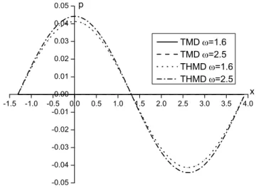
TMD =1.6 TMD =2.5 THMD =1.6 THMD =2.5
x p
-1.5 -1.0 -0.5 0.0 0.5 1.0 1.5 2.0 2.5 3.0 3.5 4.0
-0.25 -0.20 -0.15 -0.10 -0.05 0.00 0.05 0.10 0.15 0.20 0.25
TMD =1.6 TMD =2.5 THMD =1.6 THMD =2.5
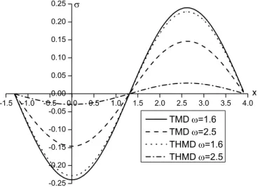
x
Figure 3: Vertical stress for z1.0 with Q0 under two methods.
-1.5 -1.0 -0.5 0.0 0.5 1.0 1.5 2.0 2.5 3.0 3.5 4.0
-3.0 -2.5 -2.0 -1.5 -1.0 -0.5 0.0 0.5 1.0 1.5 2.0 2.5 3.0
TMD =1.6 TMD =2.5 THMD =1.6 THMD =2.5
10-9
x
Figure 4: Temperature distribution for z1.0 with Q0 under two methods.
uni-formly distributed normal force, as shown in Fig. 2. The TMD values remained at zero because we did not consider the effects of the fluid in this case. This means that by only using the TMD meth-od, we were unable to assess excess pore water pressure. In actuality, many practical engineering applications are dependent on soil or saturated porous soil such as waste landfill engineering and nuclear waste management. Therefore, non-dimensional excess pore water pressure is an important physical variable in many real life applications. Figure 3 is similar to Fig. 1: As frequency increases, the difference between the two methods becomes more significant. As shown in Fig. 4, frequency has an increasing effect under both methods.
-1.5 -1.0 -0.5 0.0 0.5 1.0 1.5 2.0 2.5 3.0 3.5 4.0
-0.08 -0.06 -0.04 -0.02 0.00 0.02 0.04 0.06 0.08
=1.6
=1.8
=2.1
=2.5
w
x
Figure 5: Vertical displacement for z1.0 with Q0 under THMD method.
-1.5 -1.0 -0.5 0.0 0.5 1.0 1.5 2.0 2.5 3.0 3.5 4.0
-0.05 -0.04 -0.03 -0.02 -0.01 0.00 0.01 0.02 0.03 0.04 0.05
=1.6
=1.8
=2.1
=2.5
p
x
-1.5 -1.0 -0.5 0.0 0.5 1.0 1.5 2.0 2.5 3.0 3.5 4.0
-0.25 -0.20 -0.15 -0.10 -0.05 0.00 0.05 0.10 0.15 0.20 0.25
=1.6
=1.8
=2.1
=2.5
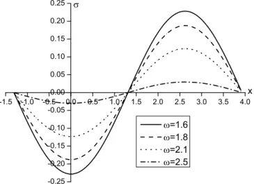
x
Figure 7: Vertical stress for z1.0 with Q0 under THMD method.
-1.5 -1.0 -0.5 0.0 0.5 1.0 1.5 2.0 2.5 3.0 3.5 4.0
-3 -2 -1 0 1 2 3
=1.6
=1.8
=2.1
=2.5
x 10-9
Figure 8: Temperature distribution for z1.0 with Q0 under THMD method.
-1.5 -1.0 -0.5 0.0 0.5 1.0 1.5 2.0 2.5 3.0 3.5 4.0
-0.12 -0.08 -0.04 0.00 0.04 0.08 0.12
=1.6
=1.8
=2.1
=2.5 w
x
Figure 9: Vertical displacement for z1.0 with q0 under THMD method.
-1.5 -1.0 -0.5 0.0 0.5 1.0 1.5 2.0 2.5 3.0 3.5 4.0
-2.0 -1.5 -1.0 -0.5 0.0 0.5 1.0 1.5 2.0
=1.6
=1.8
=2.1
=2.5 p
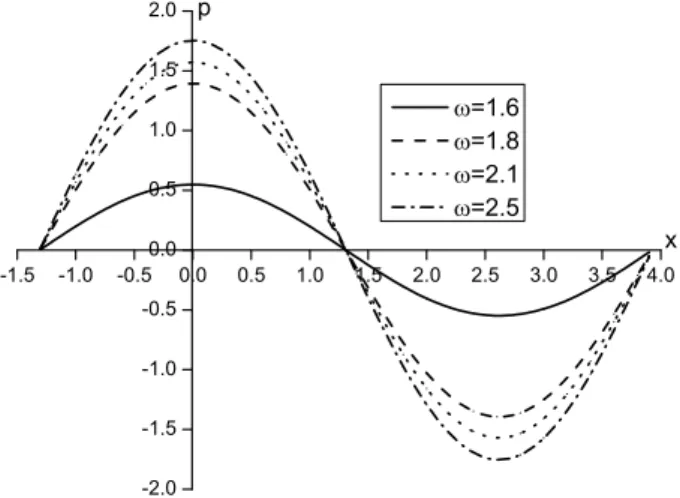
x
Figure 10: Excess pore water pressure for z1.0 with q0 under THMD method.
-1.5 -1.0 -0.5 0.0 0.5 1.0 1.5 2.0 2.5 3.0 3.5 4.0
-3 -2 -1 0 1 2 3
=1.6
=1.8
=2.1
=2.5
x
-1.5 -1.0 -0.5 0.0 0.5 1.0 1.5 2.0 2.5 3.0 3.5 4.0
-0.5 -0.4 -0.3 -0.2 -0.1 0.0 0.1 0.2 0.3 0.4 0.5
=1.6
=1.8
=2.1
=2.5
x
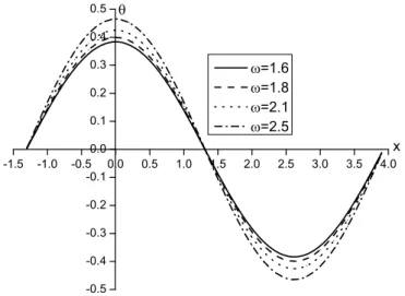
Figure 12: Temperature distribution for z1.0 with q0 under THMD method.
In the figures above (Case 3), based on the THMD method, the solid line, dashed line, dotted line, and dashed-dotted line refer to
1.6,
1.8,
2.1, and
2.5, respectively. In this case, we assumed that only a uniformly distributed thermal source was applied to the surface of the half-space. As discussed above, our research medium is saturated porous soil, where normal load mainly includes non-dimensional excess pore water pressure and non-dimensional vertical stress. In this case, only a uniformly distributed thermal source is applied and the normal load is zero. Thus, the absolute value of dimensional excess pore water pressure and the absolute value of non-dimensional vertical stress are equal. A plus or minus sign only denotes that the medium is under tension or compression. The thermal expansion coefficient of pore water is greater than the thermal expansion coefficient of solid grains. The extent to which water drains from the medium decreases as frequency increases, while non-dimensional vertical displacement, excess pore water pressure, vertical stress, and temperature distribution all increase as frequency continues to increase. The frequency has an increasing effect to all the magnitudes of all physical variables. In addition, as observed from the figures, the effect of frequency has the same change trend.6 CONCLUSIONS
In this study, we investigated the thermo-hydro-mechanical problems of a poroelastic half-space soil medium with variable properties under the theory of generalized thermoelasticity. We were able to solve these problems using normal mode analysis. Based on the numerical results, we arrived at the following conclusions:
(2)When subjected to a uniformly distributed normal force, the values of non-dimensional ex-cess pore water pressure in the TMD method are consistently zero because the effect of fluid is not considered. This means that the TMD method is not appropriate for determining non-dimensional excess pore water pressure. Non-non-dimensional excess pore water pressure is an important physical variable in real life engineering. However, fluid presence attenuates the response in terms of non-dimensional vertical displacement and vertical stress, which is espe-cially pronounced at higher frequencies.
(3)The frequency of a uniformly distributed thermal load has a pronounced effect on non-dimensional vertical displacement, excess pore water pressure, vertical stress, and tempera-ture distribution. Furthermore, as observed from the figures of Case 3, the effect of frequency has the same change trend.
(4)Frequency plays an important role in examining the deformation of the body.
(5)As shown in all figures, it can be clearly observed that the figures reveal is consistent with simple harmonic oscillation, which is mainly dominated by the intrinsic nature of the solu-tion obtained when the normal mode analysis method is applied to decouple the equasolu-tion.
References
Abbas, I.A. and Youssef, H.M. (2015). Two-dimensional fractional order generalized thermoelastic porous material, Latin American Journal of Solids and Structures, 12: 1415-1431.
Abo-Dahab, S.M., Lotfy, K.H., and Gohaly A. (2015) Rotation and magnetic field effect on surface waves propaga-tion in an elastic layer lying over a generalized thermoelastic diffusive half-space with imperfect boundary, Mathe-matical Problems in Engineering, 2015: 671783.
Abousleiman, Y. and Ekbote, S. (2005). Solutions for the inclined borehole in a porothermoelastic transversely iso-tropic medium, Transactions of the ASME. E: Journal of Applied Mechanics, 72: 102-114.
Ailawalia, P. and Singla, A. (2016). Internal heat source in a thermoelastic hydrostatically initially stressed plate immersed in a liquid, Journal of Engineering Physics and Thermophysics, 89: 1255-1264.
Bai, B. (2006a). Thermal consolidation of layered porous half-space to variable thermal loading, Applied Mathemat-ics and MechanMathemat-ics, 27: 1531-1539.
Bai, B. (2006b). Fluctuation responses of saturated porous media subjected to cyclic thermal loading, Computers and Geotechnics, 33: 396-403.
Bai, B. (2006c). Response of saturated porous media subjected to local thermal loading on the surface of semi-infinite space, Acta Mechanica Sinica, 22: 54-61.
Bai, B. and Li, T. (2009). Solutions for cylindrical cavity in saturated thermoporoelastic medium, Acta Mechanica Solida Sinica, 22: 85-94.
Bai, B. and Li, T. (2013) Irreversible consolidation problem of a saturated porothermoelastic spherical body with a spherical cavity, Applied Mathematical Modelling, 37: 1973-1982.
Bai, M. and Abousleiman, Y. (1997). Thermoporoelastic coupling with application to consolidation, International Journal for Numerical and Analytical Methods in Geomechanics, 21: 121-132.
Bijarnia, R. and Singh, B. (2012). Propagation of plane waves in an anisotropic generalized thermoelastic solid with diffusion, Journal of Engineering Physics and Thermophysics, 85: 478-486.
Biot, M.A. (1977). Variational Lagrangian-thermodynamics of non-isothermal finite strain mechanics of porous solids and thermomolecular diffusion, International Journal of Solids and Structures, 13: 579-597.
Booker, J.R. and Savvidou, C. (1984). Consolidation around a spherical heat source, International Journal of Solids and Structures, 20: 1079-1090.
Green, A.E. and Lindsay, K.A. (1972). Thermoelasticity, Journal of Elasticity, 2: 1-7.
Green, A.E. and Naghdi, P.M. (1991). A reexamination of the basic results of themomechanics, Proceedings of the Royal Society of London A, 432: 171-194.
Green, A.E. and Naghdi, P.M. (1992). On undamped heat waves in an elastic solid, Journal of Thermal Stresses, 15: 252-264.
Green, A.E. and Naghdi, P.M. (1993). Thermoelasticity without energy dissipation, Journal of Elasticity, 31: 189-208.
Hetnarski, R.B. and Ignaczak, J. (1999). Generalized thermoelasticity, Journal of Thermal Stresses, 22: 451-476. Kumar, R. and Devi, S. (2008). Thermomechanical intereactions in porous generalized thermoelastic material perme-ated with heat sources, Multidiscipline Modeling in Materials and Structures, 4: 237-254.
Kumar, R. and Gupta, R.R. (2010). Propagation of waves in transversely isotropic micropolar generalized thermoe-lastic half space, International Communications in Heat and Mass Transfer, 27: 1452-1458.
Kumar, R., Kaur, M. and Rajvanshi, S.C. (2014). Propagation of waves in micropolar generalized thermoelastic materials with two temperatures bordered with layers or half-spaces of inviscid liquid, Latin American Journal of Solids and Structures, 11: 1091-1113.
Liu, G.B., Xie, K.H., and Zheng, R.Y. (2009). Model of nonlinear coupled thermo-hydro-elastodynamics response for a saturated poroelastic medium, Science in China. Series E: Technological Sciences, 52: 2373-2383.
Liu, G.B., Xie, K.H., and Zheng, R.Y. (2010a). Thermo-elastodynamic response of a spherical cavity in saturated poroelastic medium, Applied Mathematical Modelling, 34: 2203-2222.
Liu, G.B., Xie, K.H., and Zheng, R.Y. (2010b). Mode of a spherical cavity’s thermo-elastodynamic response in a saturated porous medium for non-torsional loads, Computers and Geotechnics, 37: 381-390.
Lord, H.W. and Shulman, Y. (1967). A generalized dynamical theory of thermoelasticity, Journal of the Mechanics and Physics of Solids, 15: 299-309.
Lotfy, K.h. (2014). Two temperature generalized magneto-thermoelastic interactions in an elastic medium under three theories, Applied Mathematics and Computation, 227: 871-888.
Lotfy, K.h. (2016). The elastic wave motions for a photothermal medium of a dual-phase-lag model with an internal heat source and gravitational field, Canadian Journal of Physics, 94: 400-409.
Lotfy, K.h. and Hassan, W. (2014). Normal mode method for two-temperature generalized thermoelasticity under thermal shock problem, Journal of Thermal Stresses, 37: 545-560.
Lu, Z., Yao, H.L., and Liu, G.B. (2010). Thermomechanical response of a poroelastic half-space soil medium subject-ed to time harmonic loads, Computers and Geotechnics, 37: 343-350.
Ram, P., Sharma, N. and Kumar, R. (2008). Thermomechanical response of generalized thermoelastic diffusion with one relaxation time due to time harmonic sources, International Journal of Thermal Sciences, 47: 315-323.
Schanz, M. (2009). Poroelastodynamics: linear models, analytical solutions, and numerical methods, Applied Mechan-ics Reviews, 62: doi:10.1115/1.3090831.
Sherief, H.H. and Hussein, E.M. (2012). A mathematical model for short-time filtration in poroelastic media with thermal relaxation and two temperatures, Transport in Porous Media, 91: 199-223.
Singh, B. (2007). Wave propagation in a generalized thermoelastic material with voids, Applied Mathematics and Computation, 189: 698-709.
Singh, B. (2016). Wave propagation in a rotating rransversely isotropic two-temperature generalized thermoelastic medium without dissipation, International Journal of Thermophysics, doi: 10.1007/s10765-015-2015-z.
Smith, D.W. and Booker, J.R. (1993). Green’s functions for a fully coupled thermoporoelastic material, International Journal for Numerical and Analytical Methods in Geomechanics, 17: 139-163.
Tzou, D.Y. (1995). A unified field approach for heat conduction from macro to micro scales, ASME Journal of Heat Transfer, 117: 8-16.
Wei, W., Zheng, R.Y., Liu, G.B., and Tao, H.B. (2016). Reflection and refraction of P wave at the interface between thermoelastic and porous thermoelastic medium, Transport in Porous Media, 113: 1-27.