David Manta and Rodrigo Gonçalves

Lisbon, Portugal, July 24-27, 2018

A GEOMETRICALLY EXACT KIRCHHOFF BEAM FINITE

ELEMENT WITH TORSION WARPING

David Manta* and Rodrigo Gonçalves*

* CERIS and Departamento de Engenharia Civil, Faculdade de Ciências e Tecnologia Universidade Nova de Lisboa 2829-516 Caparica, Portugal

e-mails: d.manta@campus.fct.unl.pt, rodrigo.goncalves@fct.unl.pt

Keywords: Geometrically exact beams; Kirchhoff beams; Torsion warping; Beam finite elements.

Abstract. In this paper, a geometrically exact beam model is presented that includes the Kirchhoff constraint and torsion-related warping, aiming at capturing accurately the flexural-torsional behaviour of slender thin-walled beams undergoing large displacements. The cross-section rotation tensor is obtained from two successive rotations: a torsional rotation and a smallest rotation to the tangent vector of the beam axis. Noteworthy aspects of the proposed formulation are the following: (i) the equilibrium equations and their linearization are completely written in terms of the independent kinematic parameters, (ii) torsion-warping is allowed, as well as Wagner effects, and (iii) arbitrary cross-sections are considered, namely cross-sections where the shear centre and centroid do not coincide. The accuracy and computational efficiency of the finite element implementation of the proposed model is demonstrated in several numerical examples involving large displacements.

1 INTRODUCTION

Geometrically exact beam models usually describe the cross-section position independently of its orientation, as in the pioneering works of Reissner [2,3] and Simo [4], and subsequently followed by many authors (e.g., [5–11]). However, for slender beams, shear deformation may be discarded (the Kirchhoff constraint) and the cross-section orientation becomes constrained to the tangent vector of the beam axis. The advantages of employing this constraint are twofold: (i) the number of kinematic DOFs are reduced and (ii) shear locking problems are discarded a priori. However, on the other hand, the fact that the cross-section rotation is constrained complicates the kinematic relations.

The present paper presents a geometrically exact Kirchhoff beam model that captures the flexural-torsional behavior of thin-walled beams undergoing large displacements. Torsion-warping and Wagner effects are allowed for, as well as cross-sections with non-coincident shear center and centroid. A finite element is obtained by approximating the independent kinematic parameters using Hermite cubic functions. The kinematic description of the beam is similar to that introduced in [20], including (i) a warping DOF to allow for an accurate representation of the torsional behavior, namely the Wagner effect, and (ii) the Kirchhoff constraint. It should be noted that the present model is not concerned with arbitrarily large displacements, as emphasis is given to the assessment of the smallest rotation parametrization approach and its application to capture flexural-torsional deformation in thin-walled beams. In this context, the singularity of the parametrization, occurring for a rotation equal to π, is not approached and a path-independent (although non-objective) formulation is obtained.

For the notation, scalars are represented by italic letters, whereas second-order tensors, vectors and matrices are represented by bold italic letters. The derivatives with respect to the coordinates Xi (i=1,2) are indicated by ( ) ,i, and the derivative with respect to X3 is represented by a prime ( ) ' . Virtual and incremental/iterative variations are denoted by δ and Δ, respectively. The tilde ã indicates a skew-symmetric second order tensor whose axial vector is a. The standard tensor, vector and scalar products between two vectors a and b are indicated by



a b, a b and a b , respectively, and the vector norm is || ||a  a a .

2 THE GEOMETRICALLY EXACT THIN-WALLED BEAM MODEL 2.1 Kinematic description

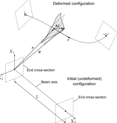
Let (X1, X2, X3) define an orthonormal direct reference system, with base vectors Ei (i=1,2,3), where the X3 axis defines the beam initial longitudinal axis, coinciding with the line of cross-section shear centers C (the beam is initially straight). According to Figure 1, the initial configuration is defined by the position vector of each material point X = X1E1+ X2 E2 + X3 E3, with X3



For the deformed configuration, the position vector of each point is given by as

1 2 3 3 3

(X ,X ,X ) (X ) (X )

x r  l, (1)

where vector r references the cross-section center C, Λ is the cross-section orthogonal rotation tensor about C and l references each cross-section point with respect to C in the co-rotational frame ΛEi, reading

2

1 1 2 ( 1, 2) ( 3) 3

X X  X X p X

  

l E E E , (2)

where ω is the torsion-related warping function and p is its scalar weight function.

With the Kirchhoff constraint, with null warping (p = 0), the cross-section remains perpendicular to the beam axis and the rotation tensor satisfies

3 

E t

 , (3)

where t is the unit tangent vector of the beam axis, defined as

. || ||

 



r r

The parametrization of the rotation tensor that satisfies Eq. (3) is discussed in Section 3.

Figure 1: Initial and deformed configurations of the beam.

2.2 Strain

The standard deformation gradient F  x is first written as follows

2 3 3

1 1 2 )

( 

    

F  g E g E g E , (5)

where T

i  i

g  FE are the back-rotations of the base vector push-forwards, FEi. From Eqs. (1) and (2), these vectors are given by

1 1,1p 3

g E E , (6)

2  2,2p 3

g E E , (7)

3   3K p' 3

g  E l E , (8)

where the material strain measures introduced by Simo [4] have been employed, reading

3

' T

 r E

  , (9)

axi( T ')



K   , (10)

with Γ relating to the beam axis extension/shearing and K measuring its curvature.

Using Eqs. (3) and (4), only the extensional component (along E3) of Γ is non-null, as one obtains

3 3 3

' || ' || (|| ' || 1)

T T

 r E  t r E  r  E

The Green-Lagrange strains _ 1₂( T _ )

E F F 1 are obtained from the previous relations. The relevant components can be cast in a Voigt-like vector form as

1

33 2 3 3

31 1 3

2 3 32 1) ( 2 2 E E E          _{ }_  _    _  _    g g

E g g

g g

. (12)

2.3 Equilibrium equations and their linearization

From the virtual work principle, using Green-Lagrange strains E and second Piola-Kirchhoff stresses [ 33 31 32]

T

S S S



S , the equilibrium equations are obtained, reading

0 e

int xt

W W

   , (13)

d int

V

W V

 



ext W

 u Q  M, (15)

where V is the beam initial volume, Q is a concentrated force and u x X is its work- -conjugate displacement, M is a concentrated moment about fixed axes and  is the spatial spin vector (see, e.g., [21]), given by

δ̃ϖ  T

. (16)

The virtual variation of the strains is given by

3 3

1 3 1 3

2 3 2 3

           _   _         g g

E g g g g

g g g g

. (17)

A linear constitutive law is assumed between S and E, reading

E G G      _{  }    

S CE E, (18)

where E is Young’s modulus and G is the shear modulus.

The incremental/iterative linearization of the virtual work equation reads

) d ( int V W V   

 

_

ext W

  

In Section 4, these equations are written explicitly in terms of the independent kinematic parameters, which follow from the choice of the cross-section rotation parametrization, discussed in the next Section.

3. PARAMETRIZATION OF THE CROSS-SECTION ROTATION 3.1 The cross-section rotation

As proposed in [1], the cross-section rotation tensor  is obtained from the composition of two successive rotations



t

    . (21)

The first rotation  consists of a torsion rotation and may be parametrized using a rotation vector φE3, where φ is the rotation angle. Using the Rodrigues formula (see, e.g., [23]), this leads to

3 3 3 3 3

sin cos ( )

 E   E E E E

   . (22)

The second rotation t corresponds to the smallest rotation between E3 and t which, as shown in Figure 2(a), may be represented by a path along the geodesic that connects the two vectors (in the figure, the corresponding rotation vector is ). This rotation tensor may be given by two alternative expressions [14]

3

t  t

   Ẽ3×t 3 3

3 ( ) ( ) 1 t     

E t E t

, (23)

 t

 +Ẽ3×t +(E3×t)

̃ _(E

3×t)

̃

1+t₃ . (24)

This parametrization is singular at t = −E3, corresponding to a rotation ||θ|| = π, which is of minor relevance for the problems addressed in this paper, as previously mentioned.

3.1 Curvatures and spin

From (10), the axis curvature may be decomposed as follows

axi( T T( )) T

' ' 

    

 _{t t}  _t  t

K        K K , (25)

axi( T )

'



t _{t t}

K   , (26)

3

axi( T ) ' '

  _{ } 

K   E , (27)

where the relation ( T) a ã

   was used (a is an arbitrary vector) and ' represents the torsion curvature due to . The derivation of an explicit expression for Kt is not straightforward. After several manipulations [26], one arrives at

3 3 3 3 3 ( 2 ( ) ) ( ) 1

B Kt '

t    _    _      t t E E t

where the bending and torsion components are given by 3 3 3 ) ( ) ( ( ) 1 B t ' '       

t t t E t t t E

K , (29)

3 3 3 ) ( 1 t ' K t   

  t t E . (30)

Note that (30) shows that torsion curvature is developed if (t t ') E₃0, which occurs if t' does not lie in the plane defined by t and E3, i.e., if there is a change in the geodesic between adjacent cross-sections. The total torsion curvature is given by the sum of (27) and (30). For illustrative purposes, Fig. 2(b) shows the evolution of the cross-section triad tEi for two distinct configurations of a 10 m length beam, which have the same end cross-section tangents and are characterized by  0. Path I corresponds to r(X32/ 2L)E1(X32/L)E2X3E3 and

in this case t' travels along a geodesic, not inducing torsional curvature. Path II is given by

3 2 2

3

3 1 3 2 3

(X / 3L) (X /L) X

  

r E E E and generates torsional curvature, as shown in the graph. Note that Kt3 generally changes under rigid-body rotations. As pointed out in [19], although

 could be prescribed to compensate for the change in Kt3 due to the rigid-body rotation, Eq. (30) is a rather complex function and cannot be accurately matched by a standard interpolation of , rendering the formulation non-objective. Nevertheless, this problem is reduced as the finite element length is decreased and/or the interpolation functions of  are enhanced.

As for the spatial spin, from the rotation, by , of (27), (29) and (30) and changing the derivative, one obtains

3 3 ) ( 1 t           E t t t t t t

 . (31)

4. A TWO-NODE BEAM FINITE ELEMENT

The finite element implementation of the proposed formulation is obtained by interpolating the displacement of the beam axis rX3E3, the rotation  and the warping weight function p. The independent kinematic parameters are collected in vector



p             r

 . (32)

Due to the Kirchhoff constraint, slope continuity is required for the displacement of the beam axis and thus standard Hermite cubic functions are employed. Although this is not required for

Figure 2: (a) Parametrization of the cross-section rotation and (b) evolution of the cross-section orientation along two paths with coinciding end tangents (path II yields torsion curvature).

The equilibrium equations and their linearization are written in terms of the kinematic parameters in



' ''

           

  

as the equations are written in terms of  and . In particular, the internal virtual work (14) may be written as

d T T D int V W V

  

_

3 3 1 3 2 3 1 2 3 3 [ ] [ ] [ ] [ ] [ ] T D T T

D D D

T T D D     _  _  _    g

E g g

g g g g g g g       . (35)

Its linearization reads

2 ( )) d

T T D D int V D W V   

 



E

C S

     , (36)



 







2 2 2

3 3 3 1 3 3 1 3

2 2 3 3 2 ₃

33 3 13 1

23 2

) ( ) ( )

( (

)

T T T

D D D D D D

D D D

T T

D D D D D

S S

S

    

  

g g g g g g

E g g

g g g g g

g g

g S

        

     . (37)

For the external virtual work (15) one has for the force contribution

 

D ext

W

  Q  x, (38)

2 ex T D t W  

   _x. (39)

The contribution of the moment is

 

ext

T

W 

  M _, (40)

ex

T t

W _

  

   , (41)

As explained in [26], the matrices D() and D2() are symmetric, except  and , which

are not symmetric due to the fact that the moment is not conservative.

The element tangent stiffness matrix is obtained from Eqs. (36), (39) and (41), the external force vector is obtained from (38) and (40), whereas the internal force vector follows from (34).

5. NUMERICAL EXAMPLES

5.1. Cantilever beam subjected to rotating tip loads

Consider the rectangular section cantilever beam shown in Figure 3, subjected to a free end centroidal force F = 100 kN. The force is first applied downwards ( = 0), in a single step, and then its direction is changed by multiples of 45º, while the intensity is maintained. The beam is discretized with four equal-length finite elements and infinitesimal strains are considered, meaning that the proposed formulation may be compared with the Euler-Bernoulli model.

first equilibrium iteration. The figure shows the deformed configurations for each load increment and the evolution of the norm of the out-of-balance forces corresponding to M3 and F only, designated by ||T||, with the accumulated number of iterations. Naturally, during the iterations of the first increment no torsion is generated, since all cross-sections are orientated along the same geodesic, and thus no values are shown in the graph for iterations 1 to 6. For the subsequent increments, torsion appears but decreases as the iterative process progresses. For all increments, a radial displacement of the tip equal to 3.00711803 m was obtained after six iterations.

Figure 3: Cantilever subjected to a rotating tip force. The deformed configurations are obtained by subdividing each finite element into four segments.

Figure 4 shows the results obtained when a free end moment is applied instead. Once again, no torsion occurs in the first increment but is generated in the subsequent increments (and decreases as the corresponding iterations progress). For all increments, the radial displacement of the tip equals 3.51978061 m after seven iterations, which is very close to the Euler-Bernoulli solution (3.51984934 m). The bottom graph shows the error norm proposed in [19] as a function of uniform mesh refinement, for the first load increment. This norm reads

2 2

ref

x 0

3 ma

|| 1

|| || || d L

e X

u

where r corresponds to the finite element solution, rref is the reference solution (Euler-Bernoulli) and umax is its maximum displacement. The convergence rate is of order 4, as explained in [19].

Figure 4: Cantilever subjected to a rotating tip moment. The deformed configurations are obtained by subdividing each finite element into four segments.

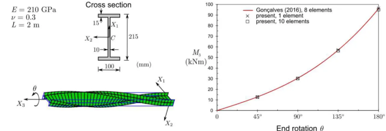
5.2. I-section under non-uniform torsion

also shown in the figure, using eight equal-length two-node shear deformable geometrically exact beam finite elements based on shell-like membrane/bending stress resultants.

The cross-section is subdivided into three walls (two 10015 flanges and one 18510 web) and the following approximate warping function is adopted (calculated assuming thin walls)

top flange X X1 2 X h2

   , (43)

web X X1 2

   , (44)

bottom flange X X1 2 X h2

   , (45)

where h h tf , with h = 215 mm and tf = 15 mm.

The results show that, due to the Wagner effect (see, e.g., [22]), a non-uniform moment-rotation relation is retrieved and axial shortening of the beam occurs. Note that a single element already leads to very accurate results and. With 10 elements and an end rotation of π, the moment is only 1.5% lower than that obtained with one element and 1.0% below that of [24].

Figure 5: I-section cantilever subjected to a torsional twist. The deformed configuration corresponds to a discretization with 10 finite elements and is rendered using four subdivisions along each wall.

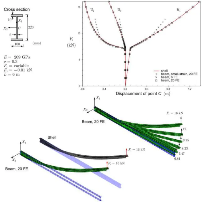
5.3. Lateral-torsional buckling of an I-section cantilever

Consider the I-section cantilever shown in Fig. 6, which undergoes lateral-torsional buckling. Besides the increasing free end shear centre force, a constant lateral perturbation force F2 = 0.01 kN is introduced to enforce a slight imperfection.

With the proposed beam element, both infinitesimal and finite strain formulations are considered. For comparison purposes, the results obtained with a refined MITC-4 shell finite element model, analysed with ADINA [25], are also provided in the figure.

Figure 6: Lateral-torsional buckling of an I-section cantilever. For the beam deformed configurations, each element is subdivided into four segments.

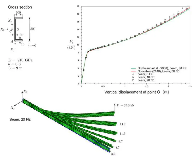
5.4. Channel cantilever beam

Finally, the lateral-torsional buckling problem of a channel section cantilever, originally proposed in [8], is analyzed. The beam is subjected to a concentrated force, applied at point A of the free end cross-section, as displayed in Figure 7. This example was selected due to the fact that, for this cross-section, the centroid and shear centre do not coincide and the force is eccentric with respect to C. In Figure 7, the results obtained with the proposed beam finite element are compared with those in [8], obtained using 30 equal-length two-node beam elements1_{, and also those obtained in [24],with 30 equal-length two-node shear deformable} geometrically exact beam elements.

1

With the proposed beam element, the cross-section is subdivided into three walls (two 10016 flanges and one 26810 web) and the following approximate warping function is adopted

top flange X2(X1 h) he

    , (46)

web X X1( 2 2 )e

    , (47)

bottom flange X2(X1 h) he

    , (48)

where b b tw/ 2, h h tf , with b = 100 mm, h = 300 mm, tf = 16 mm, tw = 10 mm, and

2

3 / (6 w/ w)

e b bht t stands for the distance between C and the web mid-line.

The graph in Figure 7 shows that using 10 equal-length elements already leads to results that practically match those obtained in [24], although for very large displacements the latter are very slightly above the ones originally presented in [8]. Increasing the number of elements to 30 improves slightly the results obtained for large displacements.

6 CONCLUSION

This paper presented a geometrically exact Kirchhoff beam model and the corresponding finite element implementation. The formulation employs the so-called “smallest rotation” parametrization of the cross-section orientation, whose treatment is far from trivial. Torsion-warping and Wagner effects are included, as well as force eccentricity effects and the possibility of considering cross-sections with non-coincident shear centre and centroid, to allow capturing the 3D large displacement behavior of thin-walled beams. The numerical examples presented clearly demonstrate the accuracy of the proposed beam finite element.

REFERENCES

[1] Boyer F. and Primault D., “Finite element of slender beams in finite transformations: a

geometrically exact approach”, International Journal for Numerical Methods in Engineering, 59, 669-702, 2004.

[2] Reissner E., “On one-dimensional finite-strain beam theory: the plane problem”, Journal of Applied Mathematics and Physics, 23(5), 795-804, 1972.

[3] Reissner E., “On one-dimensional large-displacement finite-strain beam theory”, Studies in Applied Mathematics, 52, 87-95, 1973.

[4] Simo J.C., “A finite strain beam formulation. the three-dimensional dynamic problem, part I”,

Computer Methods in Applied Mechanics and Engineering, 49, 55-70, 1985.

[5] Cardona A. and Geradin M., “A beam finite element non-linear theory with finite rotations”,

International Journal for Numerical Methods in Engineering, 26(11), 2403-2438, 1988.

[6] Pimenta P.M. and Yojo T., “Geometrically exact analysis of spatial frames”, Applied Mechanics Reviews, 46(11S), 118-128, 1993.

[7] Ibrahimbegovic A., Frey F. and Kozar I., “Computational aspects of vector-like parametrization of three-dimensional finite rotations”, International Journal for Numerical Methods in Engineering,

38(21), 3653-3673, 1995.

[8] Gruttmann F., Sauer R. and Wagner W., “Theory and numerics of three-dimensional beams with

elastoplastic material behaviour”, International Journal for Numerical Methods in Engineering,

48(12), 1675-1702, 2000.

[9] Ritto-Corrêa M., “Structural analysis of frames: towards a geometrically exact, kinematically complete and materially non-linear theory” (Ph.D. thesis), Lisbon Technical University, 2004 (In Portuguese).

[10] Gonçalves R., Ritto-Corrêa M. and Camotim D., “A large displacement and finite rotation thin -walled beam formulation including cross-section deformation”, Computer Methods in Applied Mechanics and Engineering, 199(23-24), 1627-1643, 2010.

[11] Gonçalves R., Ritto-Corrêa M. and Camotim D., “Incorporation of wall finite relative rotations in a geometrically exact thin-walled beam element”, Computational Mechanics, 48(2), 229-244, 2011.

[12]Weiss H., “Dynamics of geometrically nonlinear rods: I. Mechanical models and equations of

motion”, Nonlinear Dynamics, 30(4), 357-381, 2002.

[13] Weiss H. “Dynamics of geometrically nonlinear rods: II. Numerical methods and computational

examples”, Nonlinear Dynamics, 30(4), 383-415, 2002.

[14] Crisfield M., Non-linear finite element analysis of solids and structures, vol. 2, Wiley, 1997.

[15] Gonçalves R., “A geometrically exact approach to lateral-torsional buckling of thin-walled beams with deformable cross-section”, Computers and Structures, 106-107, 9-19, 2012.

[16]Gerstmayr J., Irschik H., “On the correct representation of bending and axial deformation in the

[17]Irschik H., Gerstmayr J., “A continuum mechanics based derivation of Reissner’s large -displacement finite-strain beam theory: the case of plane deformations of originally straight Bernoulli-Euler beams”, Acta Mechanica, 206(1-2), 1-21, 2009.

[18]Gonçalves R. and Carvalho J., “An efficient geometrically exact beam element for composite

columns and its application to concrete encased steel I-sections”, Engineering Structures, 75, 213-224, 2014.

[19]Meier C., Popp A. and Wall W.A., “An objective 3D large deformation finite element formulation

for geometrically exact curved Kirchhoff rods”, Computer Methods in Applied Mechanics and Engineering, 278, 445-478, 2014.

[20] Simo J. and Vu-Quoc L., “A geometrically-exact rod model incorporating shear and

torsion-warping deformation”, International Journal of Solids and Structure, 27(3), 371-393, 1991.

[21] Ritto-Corrêa M. and Camotim D., “On the differentiation of the Rodrigues formula and its significance for the vector-like parameterization of Reissner-Simo beam theory”, International Journal for Numerical Methods in Engineering, 55(9), 1005-1032, 2002.

[22]Pi Y.L., Bradford M.A. and Uy B., “A spatially curved-beam element with warping and Wagner

effects”, International Journal for Numerical Methods in Engineering, 63(9), 1342-1369, 2005.

[23] Goldstein H., Classical mechanics, second ed., Addison-Wesley, 1980.

[24]Gonçalves R., “A shell-like stress resultant approach for elasto-plastic geometrically exact

thin-walled beam finite elements”, Thin-Walled Structures, 103, 263-72, 2016. [25] Bathe K.J., ADINA system., ADINA R&D Inc., 2016.

[26]Manta D. and Gonçalves R., “A geometrically exact Kirchhoff beam model including torsion