Proceedings of the Annual Stability Conference Structural Stability Research Council San Antonio, Texas, March 21-24, 2017
Efficient GBT displacement-based finite elements for non-linear problems
Rodrigo Gonçalves1, Dinar Camotim2
Abstract
This paper addresses computational efficiency aspects of Generalized Beam Theory (GBT) displacement-based finite elements. It is shown that such efficiency can be significantly improved by using cross-section nodal DOFs (instead of deformation modes), since much smaller matrices need to be handled and the element stiffness matrix becomes significantly sparser. In addition, wall thickness variations, including holes, can also be considered. The deformation mode participations, which constitute the trademark of GBT, are recovered through post-processing. For illustrative purposes, several numerical examples, involving linear and non-linear (static) problems, are presented and discussed.
1. Introduction
The computational efficiency of Generalized Beam Theory (GBT3) approach in linear, buckling and free vibration problems is remarkable, since a small number of (adequately selected) cross-section deformation modes generally ensures very accurate solutions, comparable to those obtained with refined shell finite element models. In addition, the modal decomposition of the solution offers a unique insight into the mechanics of the problem under analysis and, in some cases, analytical or semi-analytical solutions can be derived. This efficiency decreases if non-linearity is present, since more modes (often large numbers) must be included in the analysis and couplings become inevitable, making it necessary to handle large matrices and leading to a dense element tangent stiffness matrix. In elastoplastic problems, some strategies were devised to minimize this problem, namely:
(i) The plastic bifurcation problem was handled by Gonçalves & Camotim (2004) and Gonçalves et al. (2010). In order to minimize mode couplings, the cross-section deformation modes were calculated using tangent elastoplastic material moduli along the pre-buckling path. The bifurcation loads were then calculated using a fast semi-analytical approach and, in addition, it was also possible to develop analytical solutions.
1
CERIS, ICIST and Universidade Nova de Lisboa, Portugal, <[email protected]>
2
CERIS, ICIST, DECivil, Instituto Superior Técnico, Universidade de Lisboa, Portugal, <[email protected]>
3
GBT is a thin-walled prismatic bar theory allowing for cross-section deformation through the consideration of a well defined set of structurally meaningful cross-section deformation modes. This theory was introduced by Schardt (1966,
1989) and has been considerably developed since it is now established as a very efficient tool for investigating
(ii) Non-linear elastoplastic load-displacement paths were obtained by Gonçalves & Camotim (2011), using a shell-like stress resultant (Ilyushin) approach, which makes it possible to avoid expensive through-thickness numerical integration and also constrain arbitrary stress/strain components to zero, thus lowering significantly the number of modes required to achieve accurate results. This approach was later extended to geometrically non-linear problems by Gonçalves & Camotim (2012).
(iii) In the work of Henriques et al. (2015, 2016), steel plasticity and concrete non-linearity were considered by setting specific stress/strain components to zero. This made it possible to employ simple material models and obtain accurate solutions for steel-concrete composite beams with a small number of deformation modes.
It is shown in this paper that the computational efficiency of GBT finite elements can be significantly improved by resorting to a “node-based” DOF approach. Although the standard GBT deformation modes are not directly included in the analyses, their participations are straightforwardly recovered in the post-processing stage. Essentially, the “node-based” GBT finite element is equivalent to an assembly of flat quadrilateral shell elements, which amounts to enhancing the standard GBT kinematic description with cross-section in-plane nodal rotations. Although these rotations increase the number of DOFs, the additional computational cost is offset by the overall efficiency of the formulation. Moreover, discrete variations of the wall thickness in the longitudinal direction (including holes4) can be easily and straightforwardly handled.
2. Standard GBT Displacement-Based Finite Elements
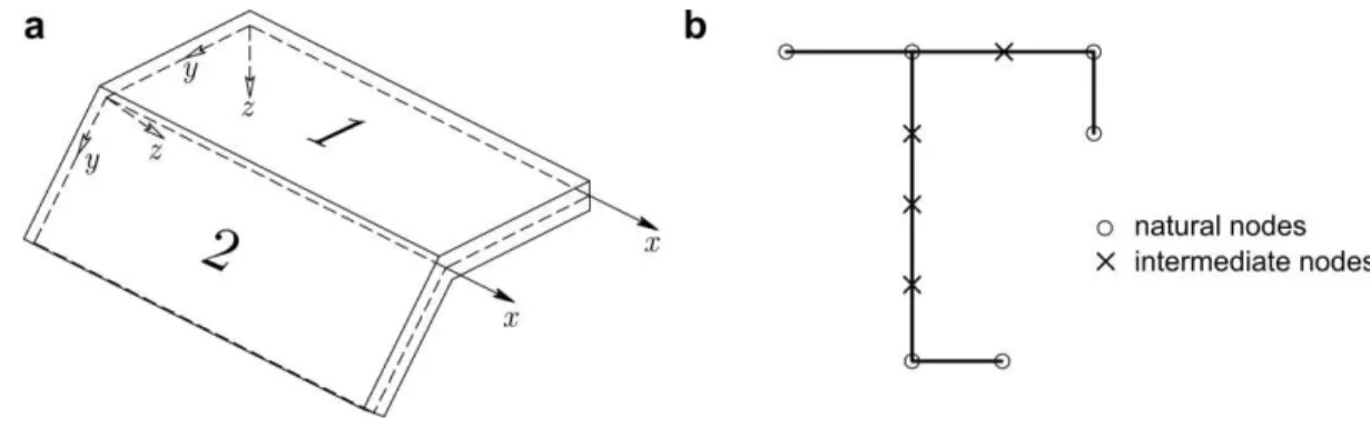
In this paper, the GBT notation and matrix formulation introduced in Gonçalves et al. (2010) and Gonçalves & Camotim (2012) is followed. Mid-surface local axes are set in each wall, as shown in Fig. 1(a), and Kirchhoff’s thin-plate assumption is enforced, making it possible to describe the beam displacements using only the wall mid-surface ones (u, v, w, along x, y, z, respectively). As usual, the beam deformed configuration is described using k=1,...,D cross-section deformation modes (shape functionsuk(y),vk(y),wk(y)), each multiplied by the corresponding amplitude function k
(unknown). The deformation mode shape functions are determined from the so-called “GBT cross -section analysis”, which involves defining a cross-section discretization (Fig. 1(b)), is described elsewhere (Gonçalves et al. 2010; 2014, Bebiano et al. 2015) and has been implemented in the GBTUL program, freely available at www.civil.ist.utl.pt/gbt.
Figure 1: (a) Wall local axes and (b) cross-section discretization.
4
In Casafont et al. (2015) and Cai & Moen (2016), the standard GBT approach is employed to handle holes, which
A plane stress state is assumed in the walls and, therefore, a reduced Voigt-like notation can be employed, with second Piola-Kirchhoff stresses ST = [Sxx Syy Sxy] and Green-Lagrange strains ET = [Exx Eyy 2Exy]. The standard GBT finite element interpolation of the amplitude functions is (x) = (x)d, where (x) is a column vector collecting the k functions, matrix (x) contains the
interpolation functions and vector d contains the unknowns. Hermite cubic polynomials are usually employed, except for the deformation modes involving exclusively warping, whose amplitude functins are approximated by Lagrange quadratic or cubic functions. For M modes involving only warping and using Lagrange quadratic functions (as done in this paper), the number of element DOFs is N = 4DM. The element internal force vector and tangent stiffness matrix read
,,
int
e e V t T G t V T dV
dV K B B CB
S B
f (1)
where Ve is the finite element volume, Ct is the tangent constitutive matrix for plane stress and B, BGare of the form
, , ,
,
, , ,
, , , , , , , 2 xx x D T xx x G xx x D Ψ Ψ Ψ w v u S Ξ Ψ Ψ Ψ B Ψ Ψ Ψ w v u φ ΞB E E (2)
where the comma indicates differentiation, u,v,w are vectors collecting the uk,vk,wkshape functions and
E E Ξ
Ξ , 2
D
D are strain-related matrices. Numerical integration is performed by means of Gauss quadrature, with 3 points along x, 3 points along y (between consecutive nodes) and at least 2 points along z (more are required in physically non-linear problems).
It is worth discussing the size of the matrices involved. Recalling that (i) D is the number of modes included in the analysis, (ii) only 3 stress/strain components are stored and (iii) N is the number of element DOFs (thus N>D), the matrix/vector sizes are
(D1), d (N1), (DN), ΞDE(33D),
E
Ξ 2
D (3D3D), B (3N), BG (NN). (3) It is clear that these matrices become quite large as the number of modes included in the analysis increases. In addition, the non-linear strains must be computed with contributions from all N DOFs, since the deformation modes generally involve displacements of the whole cross-section.
The GBT formulation is most efficient in linear elastic problems. The cross-section integration leads to the so-called GBT modal matrices B, C, D1, D2. In open sections, null membrane shear strains and null membrane transverse extensions can be assumed and the GBT mode orthogonalization procedure leads to diagonal B and C matrices and non-diagonal (but sparse) D matrices. If the
couplings in D1 and D2 are discarded, the most efficient formulation is obtained, where all modal
matrices are diagonal and a very sparse element stiffness matrix is obtained5. For arbitrary cross-sections (exhibiting closed cells) and all sets of deformation modes, couplings occur and the stiffness matrix becomes denser. It is also worth noting that the modes are calculated through a numerical
5
See also Gonçalves & Camotim (2015), where the particular cases of symmetric or periodic open sections are
procedure and, therefore, most off-diagonal matrix components are not exactly zero, rendering the identification of the relevant couplings a quite difficult task.
In physically non-linear problems, numerical integration must be carried out within an iterative solution. With P integration points in a finite element, one must handle, in general, P distinct B
matrices of dimension 3N. In addition, couplings occur and Kt becomes dense. In geometric
non-linear problems, the BG and strain-displacement matrices are also involved, which further
increases the computational cost of the analysis.
3. The Node-Based Approach
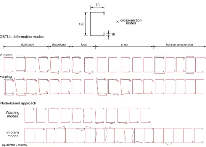
Alternatively, a node-based approach can be devised, where all wall segments are treated equally. The polynomial degrees of the modal displacement functions of the standard GBT approach are maintained, but the warping displacements are enhanced with a quadratic function: Hermite cubic functions for w and quadratic hierarchical functions for u,v , leading to 10 shape functions (“deformation modes”) in each wall segment. Naturally, it is possible to consider only part of these functions, as shown in Section 4.
Fig. 2 shows the deformation modes of a lipped channel, obtained with GBTUL and the node-based approach, for a cross-section discretization involving 6 nodes. With GBTUL, as in the standard GBT approach, the in-plane rotations are statically condensed and only linear functions are adopted for
v ,
u , leading to 18 modes. With the node-based approach, 34 modes are obtained instead.
After performing the structural analysis, the standard GBT deformation modes are recovered through a change of basis, using the inverse of the transformation matrix T, whose columns contain the components of the standard GBT deformation modes in the node-based basis. Since the node-based approach generally yields a larger number of modes, columns pertaining to the missing modes must be added to the matrix.
With the proposed approach, the matrices for a single wall segment can be employed to assemble the complete finite element matrices, using natural coordinates. The interpolation scheme for the amplitude functions k follows that of the standard approach. For a single wall segment, M = 3 and
D = 10, leading to N = 4D M = 37 DOFs. This wall segment element is quite similar to the classic Bogner-Fox-Schmit plate element (Bogner et al, 1966), but enhanced with added quadratic membrane displacements, except for the longitudinal interpolation of the v displacements, which employs Hermite cubic polynomials.
It is important to compare the node-based and standard GBT approaches, where orthogonalized modes are used (generally involving displacements of the whole cross-section). For simplicity, consider an unbranched cross-section with n walls (n+1 nodes) and assume that, in the standard GBT procedure, (i) linear and quadratic functions are employed for u,v, as in the node-based procedure, and (ii) the cross-section in-plane rotations are statically condensed (as in the classic GBT):
(i) In the standard GBT approach, M = 2n + 1, D = 5n + 3 and N = 4D M = 18n + 11. One should expect a NN dense element stiffness matrix. Furthermore, with p integration points in each wall, the total number of points in the element is P = np and, therefore, np distinct
B matrices of dimension 3(18n+11) must be handled (more matrices in geometrically non-linear problems).
(ii) The node-based approach requires handling only p distinct B matrices of dimension 337. In addition, the stiffness matrix is significantly sparse (increasingly sparse as the number of walls increases), even in non-linear problems.
Finally, a few words concerning the cross-section refinement. In the standard GBT approach, this is achieved by adding intermediate nodes. If this is done only in some elements, the additional modes must be constrained at the nodes between elements with different discretizations. However, adding intermediate nodes can change the deformation mode shapes and, if this is the case, appropriate constraint equations must be provided. In alternative, the same (refined) cross-section discretization can be employed for all elements of the bar, while eliminating some modes in specific elements. This procedure has the drawback of not reducing the number of wall segments. On the other hand, in the node-based approach, the cross-section refinement corresponds to a straightforward subdivision of the walls along y (standard h-refinement). For refinements in some elements only, hanging nodes appear between elements and the corresponding DOFs must be constrained in the usual way (Ainsworth & Senior 1997).
4. Numerical Examples
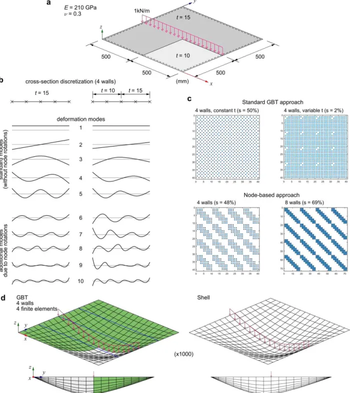
4.1 Plate with Non-Uniform Thickness
Consider the simply supported square plate shown in Fig. 3(a), with non-uniform thickness and subjected to a line load. A linear analysis is performed and, therefore, it suffices to consider
k
w modes. The plate is analyzed as a beam whose longitudinal axis x is parallel to the line load.
Figure 3: Simply supported plate with non-uniform thickness (a) geometry, loading and material properties, (b) GBT deformation modes, (c) pattern of the element stiffness matrix and (d) deformed configurations (the GBT configurations
With the standard GBT approach, the cross-section deformation modes depend on the plate stiffness and, therefore, different modes are obtained for x < 500 and x > 500 mm see Fig. 3(b), which shows the two mode sets for a cross-section subdivision into four walls (5 modes). It should be noted that the two sets do not define the same function space and it is not possible to ensure compatibility at x = 500 mm. Two solutions are possible: (i) the same deformation modes are used throughout the “beam” (in this case additional modes are required to capture the effect of the varying thickness) or (ii) cross-section nodal rotation DOFs are included, which leads to the additional modes 6-10 shown in Fig. 3(b), and compatibility equations must be set up between elements, at x = 500 mm. In contrast, in the node-based approach compatibility is ensured and the element stiffness matrix is generally sparser, as shown in Fig. 3(c) (the dots correspond to non-null components and s is the number of zero-valued elements divided by the total number of elements):
(i) The top two matrices were obtained using the standard GBT approach, by calculating first the GBT modal matrices and setting to zero the components with very small values (thus,
B and C are effectively diagonal). When the thickness is constant, sparse D1 and D2
matrices are obtained due to the fact that the modes are symmetric/anti-symmetric (see Fig. 3(b)), and the element stiffness matrix turns out to be sparse. However, when the thickness varies, dense D1 and D2 matrices are obtained (although B and C remain diagonal) and the
element stiffness matrix becomes very dense.
(ii) The bottom two matrices correspond to the node-based procedure and were calculated assuming variable thickness (with constant thickness the block bandwidth is maintained). With four walls, the sparsity is similar to that obtained with the standard approach with constant thickness, but increases as the number of walls grows (as expected).
Fig. 3(d) shows the deformed configurations obtained with the node-based GBT finite element (4 walls and 4 elements) and a shell model. The vertical displacement at the center of the plate equals 0.1409 mm (shell) and 0.1404 mm (GBT), which constitutes an excellent agreement.
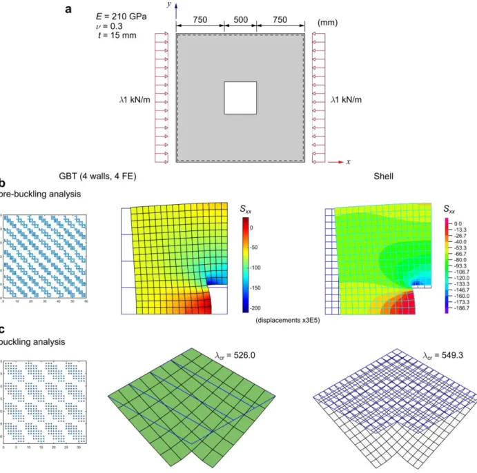
4.2 Buckling of a Plate with a Central Rectangular Hole
The critical buckling load of a simply supported square plate with a central square hole is determined next (see Fig. 4(a)). A linearized buckling analysis is performed, i.e., the influence of the pre-buckling displacements is discarded. Due to the problem double symmetry, only one quarter of the plate is analyzed. With the node-based GBT approach, the central hole is considered by setting the thickness to zero and eliminating the DOFs associated with null stiffness. The pre-buckling analysis is performed with the membrane DOFs only, whereas the buckling analysis is carried out with the out-of-plane displacements w only. In all cases, a subdivision into 4 walls and 4 elements is considered. The GBT and shell model pre-buckling analysis results for = 1 are compared in Fig. 4(b) a very good agreement is found. The stiffness matrix of the first element (0 x 250 mm) is displayed in the figure, making it possible to observe its rather sparse pattern. The critical buckling loads and corresponding mode shapes are shown in Fig. 4(c). The GBT critical load is within 4.3% of the shell model value and the buckling modes are very similar. It should be noted that, in this particular example, all pre-buckling stress components must be considered, since a GBT analysis discarding the Syy and Sxy stresses leads to cr = 480.9, significantly below the correct value. Finally,
Figure 4: Simply supported square plate with a central hole: (a) geometry, loading and material constants, (b)
pre-buckling and (c) pre-buckling analyses results (the GBT configurations are obtained with two subdivisions along x/y per
wall/element).
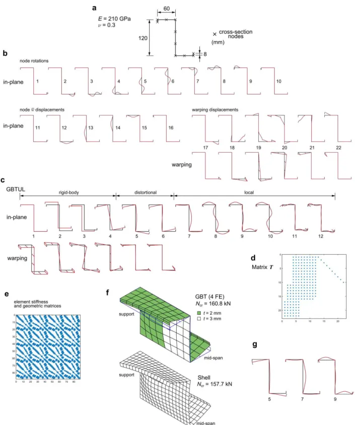
4.3 Buckling of a Lipped Zed-Section Column with a Stepped Web Thickness Variation
Although this approach leads to a stiffness matrix denser than that associated with the pure node-based approach, less deformation modes are needed to achieve accurate results.
Figure 5: Lipped zed-section column: (a) geometry, material constants and cross-section discretization, deformation modes for
the (b) node-based and (c) standard GBT approaches, (d) transformation matrix T and buckling results: (e) element linear and
For comparison purposes, the standard rigid-body, distortional and local deformation modes, obtained with GBTUL, are displayed in Fig. 5(c). These modes also satisfy the null membrane shear strain and null transverse extension assumptions. Since nodal rotations do not constitute independent DOFs, less deformation modes are obtained (less 10 modes in this case, equaling the number of nodes). A linearized buckling analysis is performed for a 300 mm length member with a 2 mm wall thickness. In this case, the GBT semi-analytical approach can be employed, as implemented in GBTUL. With the 12 deformation modes shown in Fig. 5(c) it is possible to obtain Ncr = 126.3 kN and the
associated buckling mode is characterized by a dominant participation of the distortional mode 5 (94.1%), a small participation of the local mode 7 (5.2%) and negligible participations of the remaining modes. If the analysis is performed with modes 5 and 7 only, one obtains Ncr = 127.2 kN,
which virtually coincides with the previous value.
Although the node-based approach requires the consideration of additional deformation modes (22 instead of 12), the buckling load obtained is the same (126.3 kN). This highlights the computational efficiency of the standard GBT approach: in a wide range of cases (such as the present one), only a few deformation modes (two in this case) suffice to obtain accurate results. Of course, this is not possible with the node-based approach, since all deformation modes need to be considered. To recover the participations of the standard deformation modes, the transformation matrix is employed (see Fig. 5(d)) and, naturally, the values obtained with GBTUL are retrieved.
Consider now that the web thickness is increased to 3 mm for 75 < x < 225 mm. This stepped thickness change, which canot be easily modeled with the standard GBT approach, is straightforwardly handled by the proposed node-based approach. Due to the problem symmetry, only half of the column is modeled and four equal-length finite elements are adopted, i.e., the increased web thickness appears in two elements only. The element linear and geometric stiffness matrices display the pattern shown in Fig. 5(e): they are still rather sparse, despite the fact that a partial node-based procedure was employed (some modes involve displacements of more than two consecutive walls). The buckling load increases to 160.8 kN, a value matching quite accurately the shell model result (157.7 kN). The corresponding buckling modes are displayed in Fig. 5(f), showing a distortional-type buckling with the web region of increased thickness experiencing much less plate bending.
Finally, for illustrative purposes, the modal participations at mid-span are calculated using the transformation matrix. As expected, the distortional mode 5 has a dominant participation (90.4 %), followed by the local modes 7 (7.5 %) and 9 (1.8 %) Fig. 5(g) shows the in-plane shapes of these deformation modes. The remaining modes have negligible participations.
4.7 Elastoplastic Collapse of a Lipped Channel Column
Figure 6: Lipped channel column: (a) cross-section geometry and material constants, deformation modes of the (b) standard and (c) node-based GBT approaches, (d) element tangent stiffness matrices, (e) elastoplastic deformed
This problem was first analyzed by Gonçalves & Camotim (2012), considering the standard GBT deformation modes plus additional modes accounting for linear warping and linear/quadratic v displacements, leading to the 22 modes displayed in Fig. 6(b) Fig 6(a) shows the cross-section discretization adopted, which accounts for the cross-section symmetry. The node-based approach, using the same cross-section discretization, leads to the 32 modes displayed in Fig. 6(c). The elastoplastic analyses are carried out with a stress resultant (Ilyushin) formulation, which avoids the expensive through-thickness numerical integration (see Gonçalves & Camotim 2012). For comparison purposes, elastic and elastoplastic results taken from this reference are also provided in the figure. Fig. 6(d) makes it possible to compare the patterns of the element tangent stiffness matrix obtained in a typical iteration with the standard (Gonçalves & Camotim 2012) and node-based approaches. It is once again concluded that the node-based approach leads to a much sparser matrix and it should also be noted that the standard approach matrix is not fully populated because the deformation modes in Fig. 6(b) are not fully orthogonalized and, therefore, do not involve displacements in all walls (e.g., each of the quadratic v modes 18-22 involves only displacements in a single wall). Nevertheless, it should be stressed that the node-based approach involves much less and much smaller matrices: in this case, the standard approach leads to D = 22, M = 6, N = 82 and np = 45 (5 walls and a 33 integration point grid).
The top graph in Fig. 6(f) shows the load-displacement paths obtained (i) by Gonçalves & Camotim (2012), corresponding to a refined shell model and the standard GBT approach with the 22 modes shown in Fig. 6(b), and (ii) with the proposed node-based approach and an identical longitudinal discretization. For large displacements, the latter yields results that are slightly better than those of the standard GBT approach, since more deformation modes are considered (32 instead of 22). Note also that the stress-based formulation yields better results near the peak load, since the Ilyushin yield function cannot capture accurately the onset of yielding due to bending (see the discussion in Gonçalves & Camotim 2012)). The bottom graph shows the modal participations at mid-span, obtained from the node-based results. Only the participations of the rigid-body, distortional and local modes are calculated in this case. The most relevant modes are 8 (distortional) and 9 (local) and their participations vary considerably as the displacement increases. The local mode 10 has also a noteworthy participation that increases with the displacement. Finally, Fig. 6(e) shows the deformed configurations obtained with the shell model and the two GBT approaches, for a lip lateral displacement of 24 mm a very good match is observed.
5. Concluding remarks
References
Ainsworth M., Senior B. (1997). Aspects of an adaptive hp-finite element method: Adaptive strategy, conforming
approximation and efficient solvers, Computer Methods in Applied Mechanics and Engineering, 150(1) 65-87.
Bathe K.J. (2012), ADINA System, ADINA R&D Inc.
Bebiano R., Gonçalves R., Camotim D. (2015). A cross-section analysis procedure to rationalise and automate the
performance of GBT-based structural analyses”, Thin-Walled Structures, 92, 29-47.
Bogner F., Fox R., Schmit L. (1966). The generation of interelement-compatible stiffness and mass matrices by the
use of interpolation formulae”, Proceedings of 1st Conference on Matrix Methods in Structural Mechanics, Vol.
AFFDITR-66-80, 397-443.
Cai J., Moen C. (2016). Elastic buckling analysis of thin-walled structural members with rectangular holes using
generalized beam theory”, Thin-Walled Structures, 107, 274-286.
Camotim D., Basaglia C., Bebiano R., Gonçalves R., Silvestre N. (2010). “Latest developments in the GBT analysis of
thin-walled steel structures.”Proceedings of International Colloquium on Stability and Ductility of Steel Structures,
Rio de Janeiro, Brazil, 33-58 (Vol. 1).
Camotim D., Basaglia C. (2013). Buckling analysis of thin-walled steel structures using generalized beam theory
(GBT): state-of-the-art report, Steel Construction, 6(2), 117-131.
Casafont M., Bonada J., Roure F., Pastor M. (2015). GBT calculation of distortional and global buckling loads of
cold-formed steel channel columns with multiple perforations”, CD-Rom Proceedings of 8th International Conference on
Advances in Steel Structures, Lisboa, Portugal paper 18 (18 pages).
Gonçalves R., Camotim D. (2004). GBT local and global buckling analysis of aluminium and stainless steel
columns”, Computers and Structures, 82(17-19), 1473-1484.
Gonçalves R., Le Grognec P., Camotim D. (2010). GBT-based semi-analytical solutions for the plastic bifurcation
of thin-walled members”, International Journal of Solids and Structures, 47(1), 34-50.
Gonçalves R., Ritto-Corrêa M., Camotim D. (2010). A new approach to the calculation of cross-section deformation
modes in the framework of Generalized Beam Theory”, Computational Mechanics, 46(5), 759-781.
Gonçalves R., Camotim D. (2011). Generalised beam theory-based finite elements for elastoplastic thin-walled
metal members, Thin-Walled Structures, 49(10), 1237-1245.
Gonçalves R., Camotim D. (2012). Geometrically non-linear generalised beam theory for elastoplastic thin-walled
metal members, Thin-Walled Structures, 51,121-129.
Gonçalves R., Bebiano R., Camotim D. (2014). On the shear deformation modes in the framework of generalized
beam theory, Thin-Walled Structures, 84, 325-334.
Gonçalves R., Camotim D. (2015). On distortion of symmetric and periodic open-section thin-walled members,
Thin-Walled Structures, 94, 314-324.
Henriques D., Gonçalves R., Camotim D. (2015). A physically non-linear GBT-based finite element for steel and
steel-concrete beams including shear lag effects, Thin-Walled Structures, 90, 202-215.
Henriques D., Gonçalves R., Camotim D. (2016). GBT-based finite element to assess the buckling behaviour of
steel-concrete composite beams, Thin-Walled Structures, 107, 207-220.
Schardt R. (1966). Eine erweiterung der technischen biegetheorie zur berechnung prismatischer faltwerke, Stahlbau, 35,
161-171.