www.atmos-chem-phys.net/10/9993/2010/ doi:10.5194/acp-10-9993-2010
© Author(s) 2010. CC Attribution 3.0 License.
Chemistry
and Physics
Estimation of ECHAM5 climate model closure parameters with
adaptive MCMC
H. J¨arvinen1, P. R¨ais¨anen1, M. Laine1, J. Tamminen1, A. Ilin2, E. Oja2, A. Solonen3, and H. Haario3
1Finnish Meteorological Institute, Helsinki, Finland
2Aalto University School of Science and Technology, Espoo, Finland 3Lappeenranta University of Technology, Lappeenranta, Finland
Received: 26 March 2010 – Published in Atmos. Chem. Phys. Discuss.: 6 May 2010 Revised: 8 October 2010 – Accepted: 11 October 2010 – Published: 25 October 2010
Abstract. Climate models contain closure parameters to which the model climate is sensitive. These parameters ap-pear in physical parameterization schemes where some un-resolved variables are expressed by predefined parameters rather than being explicitly modeled. Currently, best expert knowledge is used to define the optimal closure parameter values, based on observations, process studies, large eddy simulations, etc. Here, parameter estimation, based on the adaptive Markov chain Monte Carlo (MCMC) method, is ap-plied for estimation of joint posterior probability density of a small number (n=4) of closure parameters appearing in the ECHAM5 climate model. The parameters considered are related to clouds and precipitation and they are sampled by an adaptive random walk process of the MCMC. The param-eter probability densities are estimated simultaneously for all parameters, subject to an objective function. Five alternative formulations of the objective function are tested, all related to the net radiative flux at the top of the atmosphere. Con-clusions of the closure parameter estimation tests with a low-resolution ECHAM5 climate model indicate that (i) adaptive MCMC is a viable option for parameter estimation in large-scale computational models, and (ii) choice of the objective function is crucial for the identifiability of the parameter dis-tributions.
1 Introduction
Atmospheric general circulation models (GCMs) consist of dynamical laws of atmospheric motions and physical param-eterizations of sub-grid scale processes, such as cloud for-mation and boundary layer turbulence. Specified parameters appear in physical parameterization schemes where some
un-Correspondence to:H. J¨arvinen ([email protected])
resolved variables are expressed by predefined parameters rather than being explicitly modeled. These are called clo-sure parameters. A simple example of such a parameter is provided by turbulent transfer in the atmosphere. In a first order closure, the transfer of a quantityq is assumed to be proportional to the gradient ofq multiplied by a fixed dif-fusion coefficient – note that a whole hierarchy of closures of different orders exists, each with different closure param-eters (Mellor and Yamada, 1974). Another example is cloud shortwave optical properties which depend on cloud optical thickness. This can be related to resolved cloud liquid water amount via the mean effective radius of cloud water droplets. If the cloud micro-physics is not resolved, the mean effec-tive radius has to be prescribed (Martin et al., 1994). The modelled shortwave radiation flux is sensitive to the spec-ified value of this parameter, and it can act as an effective ”tuning handle” of the simulated climate.
An underlying principle in climate model development is to aim at few rather than many closure parameters. In the model development process, best expert knowledge is used to define the optimal parameter values. They can be con-strained to some degree based on observations, process stud-ies, large eddy simulations, etc. but they do not necessarily represent any directly observable quantity. Additionally, pa-rameter values can depend on the discretization details, such as grid interval or choices made regarding modeling of other physical processes. This is a dilemma since observations do not provide guidance towards resolution or modeling envi-ronment dependent parameter values. In summary, the clo-sure parameters are determined such that (i) they are consis-tent with prior knowledge, and (ii) simulations prove to be realistic in posterior validation. In fact, both can be used in an iterative manner to optimize model performance.
Various approaches are available for solving the closure pa-rameter estimation problem. First, the review paper of Navon (1993) concentrates on adjoint techniques (e.g., Rinne and J¨arvinen, 1993) and stresses the questions of parameter iden-tifiability and stability. This implies that both the estima-tion method and the parameters to be estimated need to be selected carefully. Sequential state estimation in numeri-cal weather prediction aims at fitting the initial condition and model parameters to prior information and to observa-tions (e.g., Dee, 2005). Only the maximum-likelihood fit and a Gaussian error covariance are obtained from solving the tangent-linear analysis equation. If closure parameters are estimated in this framework, their values partly reflect the latest observations – this is in fact in slight contradiction to the notion that the closure parameter distributions should be stationary.
Annan and Hargreaves (2007) provide a review of the available parameter estimation methods in climate mod-elling. They also discuss the Markov chain Monte Carlo (MCMC) method and consider it too computationally expen-sive for estimating climate model closure parameters. Their treatment of MCMC is, however, somewhat restricted to the Metropolis algorithm (Metropolis et al., 1953), and recent advances in adaptive methods are not fully covered.
Jackson et al. (2008) used a stochastic optimization method, Multiple Very Fast Simulated Annealing (MVFSA), for the search of optimal closure parameters of the CAM3.1 climate model, with respect to a cost function based on multi-source observations. The search paths of the stochastic op-timizer were used to infer about the parametric uncertainty. Villagran et al. (2008) further evaluated the performance of MVFSA and compared it against different MCMC methods with a surrogate climate model. These methods included Adaptive Metropolis (AM), the Single Component Adap-tive Metropolis (SCAM) and the Delayed Rejection AdapAdap-tive Metropolis (DRAM), see (Haario et al., 2001, 2004, 2005, 2006; Andrieu and Moulines, 2006). Villagran et al. (2008) note that MVFSA may be efficient for optimization, but sta-tistical inference about the parameter distribution tends to be biased. The results were in favor of DRAM and SCAM, es-pecially in test cases with short sampling chains.
In this article, we demonstrate the use of MCMC in the context of the atmospheric general circulation model ECHAM5. A central outcome is that it is, indeed, viable to use MCMC for parameter estimation for a climate model, at least in the context of a coarse-resolution atmospheric GCM. Research methods are presented in Sect. 2, experi-mental setup and results in Sects. 3 and 4, and discussion and conclusions in Sects. 5 and 6.
2 Materials and methods
2.1 The adaptive MCMC approach
Markov chain Monte Carlo (MCMC) methods are widely used in parameter estimation and computational inverse problems. A mathematically solid way of describing the esti-mation problem is to use Bayesian approach where the mea-surements and unknown parameters are considered as ran-dom variables and the solution is described as a combination of prior information and the evidence that comes from the measurements via the objective function (i.e., the likelihood). The solution, i.e., the estimated distribution of the retrieved parameters, is known as the posterior distribution. Instead of just finding the “best estimate”, the MCMC technique simu-lates the full distribution of the solution in thendimensional model parameter space, where nequals the number of pa-rameters to be estimated.
The classical Metropolis algorithm (Metropolis et al., 1953) proceeds in two steps. In the proposal step, a can-didate value is sampled using a “proposal distribution”. In the acceptance step, the candidate value is either accepted or rejected. The Metropolis acceptance probability depends on the values of the objective function at the candidate value and the present value. If the value is accepted, it becomes the new value in the chain and if it is rejected, the chain just repeats the present value. More probable values are always accepted but there is a positive probability to accept less probable val-ues, too. In this way it is assured that the whole target dis-tribution is explored. The exact formula for the acceptance probability is selected such that the distribution of the simu-lated values converges to the target probability.
The original Metropolis algorithm is simple and straight-forward. In practice, however, an effective performance, i.e., convergence towards the correct target distribution with rea-sonably few model evaluations, may require preliminary test runs or laborious hand tuning of the proposal distribution. Such methods, however, are not easily available in case of a computationally demanding climate model like ECHAM5. Recent developments speed up the search of the proposal by using adaptive techniques that ’learn’ during the sampling process. In this article, we have applied the Delayed Re-jection Adaptive Metropolis (DRAM) algorithm. Textbook treatment of MCMC methods can be found, e.g., in Robert and Casella (2005).
2.2 ECHAM5 model and the closure parameters
Table 1.The considered sub-set of ECHAM5 closure parameters.
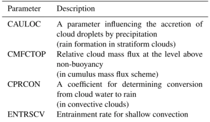
Parameter Description
CAULOC A parameter influencing the accretion of cloud droplets by precipitation
(rain formation in stratiform clouds) CMFCTOP Relative cloud mass flux at the level above
non-buoyancy
(in cumulus mass flux scheme)
CPRCON A coefficient for determining conversion from cloud water to rain
(in convective clouds)
ENTRSCV Entrainment rate for shallow convection
model vertical grid had 19 layers with model top at 10 hPa. A semi-implicit time integration scheme is used for model dynamics with a time step of 40 min. Model physical pa-rameterizations (see Roeckner et al., 2006) are invoked every time step with the exception of radiation, which is computed once in two hours.
Four ECHAM5 closure parameters were considered (Ta-ble 1). These parameters are related to physical parameteri-zations of clouds and precipitation. The choice of these pa-rameters is motivated by their substantial influence on model cloud fields and therefore the radiative fluxes at the top of the atmosphere (TOA). It is thus plausible that they can be con-strained by a suitable formulation of the objective function.
2.3 Observational data sets
In this initial study, the definition of the objective function is based solely on the net (longwave + shortwave) radiative flux at the TOA. The observational estimates are taken from the Clouds and the Earth’s Radiant Energy System (CERES) En-ergy Balanced and Filled (EBAF) dataset (Loeb et al., 2009). The CERES EBAF dataset is, however, only used for the mean values. Since this dataset contains data for five years only, we chose to derive the interannual standard deviations from the the European Centre for Medium-Range Weather Forecasts (ECMWF) reanalysis data (ERA-40; Uppala et al., 2005), which provides a much longer (44-year) timeseries.
2.4 The objective function
The parameter posterior probability distribution is condi-tional to the choice of the objective function. In case of ECHAM5, it is a measure of the accuracy of the climate sim-ulation – a trained human eye would be very efficient in se-lecting “good” and “bad” simulations and the aim here is to construct an objective function which would replace this hu-man element. On one hand, the objective function should be physically justified, i.e., being capable of distinguishing accurate climate simulations from inaccurate ones. On the other hand, it should be constructed such that the parameter
distributions are identifiable with respect to the chosen ob-jective function. If this is the case, the parameter posterior probability distribution should be compact and limited. If not, either the objective function does not provide the desired guidance for the parameters, or they are simply not relevant in tuning the model with respect to the objective function.
Five alternative formulations of the objective function are tested, all of which are related to the net radiative flux at the TOA in the ECHAM5 model (F) and in CERES EBAF data (Fo). Annual and monthly mean fluxes are denoted byF and
F, and global and zonal means byhFiand [F], respectively. Subscripts x andy refer to geographical location in zonal and meridional direction, andt refers to time (in months). The first of the five alternative formulations of the objective function is denoted byJG(θ ), and it uses only the global-annual mean value ofF:
JG(θ )=
F−Fo2
(σo
F)2
, (1)
whereθis the vector of four closure parameters. It penalizes climate simulations which deviate from the global annual-mean net radiative flux in CERES EBAF data (0.9 Wm−2). The squared net flux difference is normalized by the standard deviationσo
Fof the inter-annual variability of the global
an-nual mean net flux, which is estimated from ERA-40 data (0.53 Wm−2).
The second formulation is denoted byJXY(θ )
JXY(θ )= 1
12 12 X
t=1 X
x
X
y wx,y
Fx,y,t−Fox,y,t
2
(σo F)
2 (2)
It accounts for local differences in monthly mean net fluxes. The weights wx,y represent grid point area fractions. The
squared net flux difference is normalized by the standard de-viation of the inter-annual variability of the local monthly mean net fluxes, based on ERA-40 data. The third formu-lation, denoted byJZONAL(θ ), uses zonal mean values of monthly mean net fluxes:
JZONAL(θ )= 1
12 12 X
t=1 X
y wy
h
Fy
i
−
h
Fo y
i2
(σho
F
i)2
(3)
Here, the weightswy represent area fractions for the zonal bands, and the normalizing factor is the standard deviation of the inter-annual variability in monthly and zonal mean net fluxes.
The last two formulations
JG+XY(θ )=JG(θ )+JXY(θ ) (4)
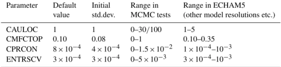
Table 2.Parameter values applied in the MCMC tests. The first column gives the default values for resolution T21L19, the second column the initial estimate of one-sigma uncertainty used to initialize the MCMC chain, the third column minimum and maximum parameter values allowed, and the fourth column the range of parameter values applied in standard ECHAM5. The upper limit of parameter CAULOC was 100 for the first four experiments, but it was reduced to 30 for theJG+ZONALexperiment, when it was realized that all values of CAULOC higher than about 30 produceidenticalresults.
Parameter Default Initial Range in Range in ECHAM5
value std.dev. MCMC tests (other model resolutions etc.) CAULOC 1 1 0–30/100 1–5
CMFCTOP 0.10 0.08 0–1 0.10–0.35 CPRCON 8×10⁻⁴ 4×10⁻⁴ 0–1.5×10⁻² 1×10⁻⁴–10−3 ENTRSCV 3×10⁻⁴ 3×10⁻⁴ 0–5×10⁻³ 3×10⁻⁴–10−3
3 Experimental setup
Five separate experiments were performed, one for each of the five objective functions listed above (Eqs. 1–5). An MCMC chain consisting of 1000 model runs was applied, with one exception: a longer chain of 4500 runs was carried out for the experiment using theJG+ZONAL objective func-tion (Eq. 5)1. Each model evaluation represents a one-year climate simulation with the low-resolution ECHAM5 model. Prescribed distributions of sea surface temperature and sea ice for year 1990 were used (AMIP Project Office, 1996), and the model initial condition was 1 January 1990. One simulation step took about 17 min using 30 CPUs on a Cray XT5m computer.
Default parameter values and prior distributions (or ranges) applied in the experiments are provided in Table 2. The MCMC algorithm was broadly as follows:
Step 0: Initialize the four closure parameters to their default val-ues; Initialize proposal distribution to reflect the a priori knowledge about parameter uncertainty; Run the model for one year; Post-process the model data and evaluate the objective function.
Step 1: Draw new parameters from the proposal distribution centered at the current parameter values; Run the model with new parameter values and evaluate the objective function.
Step 2: Accept or reject new parameter values based on the dif-ference of objective functions at current vs. previous step; Update the proposal distribution according to the adaptive MCMC algorithm.
Step 3: Return to Step 1 if the chain has not yet been completed.
1The actual length of the MCMC chain is slightly longer than the
number of ECHAM5 runs, because the parameter values proposed by MCMC may fall outside the given parameter bounds, in which case they are rejected immediately, without running ECHAM5.
Note that the difficulty in providing a correct initial pro-posal covariance in Step 0 makes the adaptation method ap-plied in Step 2 crucial for the sampling to be efficient.
4 Results
The MCMC tests with the low-resolution ECHAM5 climate model are discussed in the next four subsections, with em-phasis on general aspects of the results.
4.1 Parameter chains
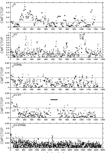
The random walk process is started in each experiment from the default parameter values (Table 2). The parameter val-ues for the subsequent runs depend on the definition of the objective function. We illustrate this by showing the MCMC chains for the five different objective functions and for two parameters with contrasting behaviour: CMFCTOP (Fig. 1) and CPRCON (Fig. 2). In Figs. 1 and 2, the dots represent pa-rameter values included in the MCMC chain. If a papa-rameter combination is rejected by the MCMC algorithm, the previ-ous accepted parameter values are repeated. The horizontal grey line represents the default parameter value, 0.1 for CM-FCTOP and 8×10⁻⁴for CPRCON, respectively. Note that in Fig. 1, the scale is different in different panels.
For CMFCTOP (Fig. 1), the parameter values are gen-erally well-bounded from above. Only for JXY the con-straint on CMFCTOP is somewhat weak, the largest accepted parameter values approaching the upper limit of physically meaningful values (CMFCTOP=1). For JG, the accepted parameter values vary on both sides of the default value, while for the three remaining cost functionsJZONAL,JG+XY
andJG+ZONAL, there is a clear tendency for parameter val-ues smaller than the default. Overall, CMFCTOP is an exam-ple of a parameter which behaves quite in an expected way.
Fig. 1.The MCMC chain for parameter CMFCTOP. The horizon-tal grey line at parameter value 0.1 is the default value. Note the different scaling in different panels. Also note that the length of the MCMC chains is slightly larger than the number of ECHAM5 runs performed (1000 for the first four chains, 4500 for theJG+ZONAL
chain).
parameter values is met. There seems to be a tendency to-wards parameter values larger than the default. Figure 2 is an example of a parameter which is weakly constrained by any of the objective functions, and the overall behaviour is not very desirable. A possible explanation is that for changes in CPRCON, the corresponding changes in longwave and short-wave fluxes at the TOA tend to cancel each other, leading to smaller changes in the TOA net flux.
In general, Figs. 1 and 2 point to the importance of the choice of the objective function. This is seen both in the fact that some objective functions constrain CMFCTOP much more tightly than others (e.g., compare JG+ZONAL with
JXY) and in the failure of all objective functions to con-strain CPRCON properly. The latter point calls for an im-proved definition of the objective function in future work. Specifically for CPRCON, compensation between longwave and shortwave fluxes suggests that an objective function that
Fig. 2.Same as Fig. 1 but for parameter CPRCON. The horizontal grey line at parameter value 8×10⁻⁴is the default value.
utilizes these fluxes separately, rather than only the net flux, might better constrain this parameter. Other model fields sen-sitive to CPRCON include precipitation rate, and middle and high cloud fractions.
Another general point evident in particular in Fig. 2 con-cerns the convergence of the MCMC chains. For exam-ple, when using the objective function JG, the values of CPRCON remain relatively close to the default value nearly until the end of the chain, but then rapidly drift to a much higher level. Had we stopped the chain after (e.g.) 800 runs, we could have falsely concluded thatJG constraints CPRCON rather well. This suggests that a MCMC chain length of 1000 runs is not long enough for analyzing the pos-terior parameter distributions properly. The issue of chain convergence is addressed more comprehensively in the fol-lowing section, based on theJG+ZONALexperiment.
4.2 Analysis of the JG+ZONALexperiment
Fig. 3. A demonstration of how the MCMC posterior distribution converges with increasing chain length for theJG+ZONAL objec-tive function. The dotted blue, black and red lines show the 10th, 50th and 90th percentiles of the posterior distribution for the previ-ous 500 runs (or for all runs performed so far, for runs 1–499). The horizontal blue, black and red lines indicate the 10th, 50th and 90th percentile of the posterior distribution computed using the last 3500 runs (i.e, runs 1001–4500) of the chain. The horizontal grey lines indicate the default values of the parameters.
evaluated the posterior distributions after each run, always
using the last 500 runs only. The blue, black and red dotted lines in Fig. 3 show the 10th, 50th and 90th percentage points computed from these distributions for each of the four param-eters. The solid horizontal lines show the respective percent-age points computed from the last 3500 runs (i.e., runs 1001 through 4500).
While the parameters start from their default values, all of them experience a drift in the early part of the chain, so that the distributions of CAULOC, CPRCON and ENTRSCV drift towards higher values and that of CMFCTOP towards lower values. By visual inspection of Fig. 3, the drift lasts for roughly 500–1000 runs, CPRCON and ENTRSCV sta-bilizing slightly earlier than CAULOC and CMFCTOP. For all parameters, percentage points computed from runs 1001– 1500 are close to those computed from runs 1001–4500. This suggests that for the analysis of the parameter posterior dis-tributions, it is sufficient to omit the first 1000 runs.
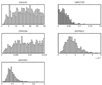
Figure 4 displays posterior distributions of the four param-eters computed from runs 1001 through 4500. As shown before (Fig. 1), for CMFCTOP there is a strong preference for values smaller than default (0.1). Also, as suggested by Fig. 2, CPRCON is poorly constrained from above. In broad terms, all values are deemed equally likely by the MCMC algorithm, except that the very lowest values are ruled out. CAULOC behaves quite similarly to CPRCON. Finally, the posterior distribution for ENTRSCV features a broad maxi-mum centred around ENTRSCV≈1.5×10⁻³. Both the low-est values and very high values of ENTRSCV are deemed
0 5 10 15 20 25 30
CAULOC
0 0.05 0.1 0.15 0.2
CMFCTOP
0 0.005 0.01 0.015
CPRCON
0 1 2 3 4 5
x 10−3 ENTRSCV
4 4.5 5 5.5 6
sqrt(costf.)
Fig. 4.Estimated posterior distributions as chain histograms for the
JG+ZONALcost function. Histogram is calculated from the chain with the first 1000 values removed. The lowest panel shows the histogram of square root of values of the cost function.
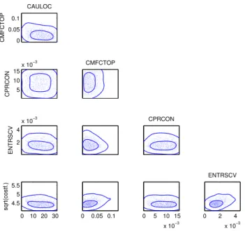
unlikely. The 2-dimensional marginal posteriors (Fig. 5) do not display significantly large correlations between the pa-rameters and further reveal the rather poor identifiability of CAULOC and CPRCON. In summary, when using the ob-jective function JG+ZONAL, the MCMC algorithm is able to providesomeconstraints on all four parameters consid-ered, although for CAULOC and CPRCON, the constraints are rather weak.
4.3 Objective function versus radiative fluxes
Trivially, parameter retuning by the MCMC process can im-prove (i.e., decrease) the value of the objective function com-pared to its value for default parameter settings. A crucial question is, however, whether the MCMC process helps to reduce errors in those quantities not explicitly included in the objective function. A simple test illustrated in Fig. 6 in-dicates that this is, again, dependent on the choice of the ob-jective function.
Figure 6 displays the five different objective functions ver-sus global annual mean net, longwave (LW) and shortwave (SW) radiative fluxes at the TOA – recall that only the net flux, rather than LW and SW fluxes separately, is used in the objective functions (1)–(5). The vertical grey line represents the observed global annual mean fluxes from CERES EBAF data, and the grey dot corresponds to the default parameter values. ForJG (Fig. 6, panels a–c), the cloud of points of the MCMC chain is exactly parabolic for net radiation, as
0 0.05 0.1
CMFCTOP
CAULOC
5 10 15
x 10−3
CPRCON
CMFCTOP
2 4
x 10−3
ENTRSCV
CPRCON
0 10 20 30 4.5
5 5.5
sqrt(costf.)
0 0.05 0.1 0 5 10 15
x 10−3
0 2 4
x 10−3 ENTRSCV
Fig. 5.Pairwise MCMC chain plots for theJG+ZONALcost func-tion. The first 1000 points are removed as burn-in time, as in the histograms of Fig. 4. The contours estimate 50% and 95% poste-rior probability levels of the marginal 2 dimensional distributions. Note that in addition to the four model parameters, the square root of value of the cost function is included as the fifth chain member.
ForJG, the default parameter values correspond to LW and SW biases of 7–8 Wm−2. It is possible to select parameter values for an unbiased model in net radiation which corre-spond to LW and SW biases in the interval of about 3 to 20 Wm−2, but not smaller. In particular, an overestimate of the (down-up) LW radiation at the TOA compared to CERES EBAF data seems to be an inherent bias of ECHAM5 at T21 resolution.
ForJXY (Fig. 6d–f), the cloud of points of the MCMC chain is diffuse and weakly parabolic for net radiation, and
JXY varies rather little from one MCMC step to another. There is a strong tendency for a positive net flux bias. Thus, minimization of errors in the geographical distribution of the monthly net flux is not a sufficiently strong constraint for obtaining correct global annual net flux. Note, however, that
JXYtends to decrease when the LW and SW biases decrease, which is a very desirable property ofJXY.
ForJZONAL (Fig. 6g–i), the main cloud of points has a weak tendency for a positive bias in the global annual net flux, implying thatJZONAL constrains somewhat better the global annual mean flux than JXY. There is a very clear tendency forJZONALto decrease when the LW and SW bi-ases decrease. The default model is somewhat outlying in the LW/SW fluxes compared to the main cloud of points.
Next, the formulationsJG+XY andJG+ZONAL, which uti-lize both the global annual net flux and the geographical dis-tribution on monthly basis, are examined. The behaviour ofJG+XY versus net radiation is largely dominated by the
Fig. 6. The objective function versus global annual mean radia-tive fluxes (net, LW, and SW). The vertical grey line represents the observed global annual mean value in CERES data (0.9 Wm−2,
−239.6 Wm−2and 240.5 Wm−2for net, LW, and SW fluxes, re-spectively), and the grey dot corresponds to the default parameter values.
global annual mean term (Fig. 6, j–l). This is mainly be-cause the normalizing factor σ is much smaller in Eq. (1) than in Eq. (2) (i.e., the global annual mean flux varies much less than local monthly mean values, and therefore provides a stricter constraint on the parameters). However, JG+XY
constrains the LW and SW parts somewhat better than JG
alone (Fig. 6a–c). Finally, the behaviour ofJG+ZONAL ver-sus net radiation is to some extent dominated by the global annual mean term (Fig. 6m–o), but the zonal net flux dis-tribution makes a significant condis-tribution. The LW and SW parts are nicely constrained such that their biases de-crease asJG+ZONAL decreases. Overall, the behaviour of
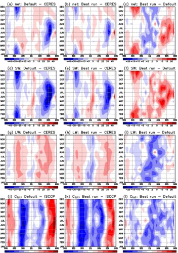
Fig. 7. Time-latitude cross section of TOA net flux difference be-tween the default ECHAM5 and CERES observations (panela), the corresponding difference for the ECHAM5 run with the smallest value ofJG+ZONAL(panelb), and the difference between these two ECHAM5 runs (panelc; note the different scale for shading).
(d)–(f): Same as (a)–(c) but for the (down-up) shortwave flux at the TOA.(g)–(i): Same as (a)–(c) but for the (down-up) longwave flux at the TOA.(j)–(l): Same as (a)–(c) but for total cloud fraction (Ctot) compared with ISCCP satellite observations. The parame-ter values corresponding to default ECHAM5 are CAULOC=1, CMFCTOP=0.1, CPRCON=8×10⁻⁴, and ENTRSCV=3×10⁻⁴; while those for the best run are CAULOC=29.83, CMFCTOP=
0.0333, CPRCON=1.05×10⁻², and ENTRSCV=1.35×10⁻³. The corresponding values ofJG+ZONALare 28.7 and 16.7.
respect to the net flux and the geographical distributions are respected to some extent.
Based on Fig. 6 (and also Figs. 1 and 2), what can we con-clude regarding the choice of the objective function? First, given that a reasonable simulation of the global annual-mean net flux at the TOA is necessary to avoid climate drift in coupled atmosphere-ocean GCMs, it seems prudent to in-clude this term explicitly in the objective function (cf. Jack-son et al., 2008). Second, use of the global-mean TOA radi-ation balance alone does not work well. It is possible to get a single number “right” with very different model climates, as
demonstrated by the wide range of global mean LW and SW radiation corresponding to low values ofJGin Fig. 6b and c. Thus, terms addressing modeled spatio-temporal struc-tures should also be included in the objective function. In this respect, use of zonal and monthly-mean values (JZONAL
andJG+ZONAL) appears a better choice than the use of lo-cal monthly-mean values (JGandJG+XY). The reason for this is that zonal values exhibit smaller interannual “random” variations than the local values (i.e., values ofσho
F
iin Eq. (3)
are substantially smaller than those ofσo
F in Eq. 2). In order
for MCMC to be able to efficiently distinguish “good” from “bad” parameter combinations, the systematic impact of pa-rameter changes needs to be relatively large compared to the random variations.
Lastly, it is by no means our purpose to imply that
JG+ZONALis the ultimate solution to the problem of defin-ing the objective function. Other model fields beyond the net flux could/should be included. Also, it should be stressed that while the use of zonal means is simple, it is hardly the opti-mal choice for the description of spatial structures. For ex-ample, the use of empirical orthogonal functions, as in Jack-son et al. (2008), is certainly an option worth considering.
4.4 Illustration of the simulation errors
Figure 7 illustrates the impact that a parameter retuning through the MCMC process has on the climate simulated by ECHAM5. Two model runs are considered: the “default run” using the default parameter setting, and the “best run” corresponding to the smallest value of the objective func-tionJG+ZONAL. The corresponding values ofJG+ZONALare 28.7 and 16.7, respectively.
For the default run, the largest net flux errors appear at high latitudes (∼55◦S and ∼60◦N) during local summer, with differences of about −40 Wm−2 from CERES EBAF data (Fig. 7a). At lower latitudes, smaller and predominantly positive biases prevail. For the optimized closure parameters (Fig. 7b), the maximum monthly mean errors are reduced by about 10 Wm−2. The pattern of differences between the two runs (Fig. 7c) is, for the most part, opposite to that of the original biases.
Finally, total cloud fraction is considered in Figs. 7j–l. Compared to the International Satellite Cloud Climatology Project (ISCCP) D2 data (Rossow et al., 1996; Rossow and Due˜nas, 2004), the default run features too much cloudiness at high latitudes, and too little cloudiness at lower latitudes, with largest negative biases around 30◦S (Fig. 7j). In the “best run”, cloudiness is, overall, reduced (Fig. 7l). While this alleviates the positive bias compared to ISCCP data at high latitudes, the negative bias prevailing over most of the globe is increased (Fig. 7k). In summary, some of the quan-tities not included in the cost function are improved, while others are deteriorated.
5 Discussion
The MCMC approach requires long chains of model runs and is therefore best applicable to models that can be run relatively fast. In the present work, we have demonstrated (as far as we know, for the first time) that it is viable to apply MCMC to parameter estimation in an atmospheric general circulation model (GCM) used for climate simula-tions. This is based on three facts: the low spatial reso-lution of the model, application of the adaptive MCMC al-gorithm (DRAM), and the relatively fast response of atmo-spheric processes to “external forcing” (in our case, changes in parameter values). As to the limits of the approach, we note that in, e.g., ocean GCMs, the response time scales are much longer and MCMC would be computationally more de-manding. Also, additional care is needed in selecting the cost function if we model systems which include important reser-voirs associated with long time scales, such as carbon pools. This is the case with comprehensive Earth system models with sub-models for terrestrial biosphere and ocean biogeo-chemistry. One can of course estimate parameters off-line for terrestrial biosphere models (Tuomi et al., 2009), for in-stance, but interactions and feedbacks with the rest of the modelling systems are omitted in this procedure.
Traditional model parameter sensitivity analysis applies perturbations on model parameters, and draws conclusions about the sensitivity of model simulations on parameter val-ues. This is typically done separately for different model parameters. This study illustrates that the range of param-eter values that can produce good simulations in terms of an objective function can be much wider when more than one parameter is considered simultaneously. This is because the combined effect of two or more parameters can keep the model simulation in an acceptable region. Traditional sen-sitivity analysis thus makes the parameter space to appear more limited than it really is. Also, it is extremely hard to find these combined effects with traditional methods.
One issue of concern with the MCMC approach is related to error compensation. The optimal values of the closure pa-rameters may depend on processes that these papa-rameters do not directly influence. For example, all-sky net radiation at
the TOA is a sum of clear-sky net radiation and cloud radia-tive forcing. Any bias in clear-sky radiaradia-tive transfer calcu-lations could influence the posterior distribution of closure parameters that affect cloudiness. The problem of error com-pensation is, however, not inherent to MCMC but applies to model retuning in general. Presumably the best way to miti-gate this problem in the framework of MCMC is to carefully select an objective function that accounts for multiple aspects of climate. Various other fields beyond the TOA net radiation could be used, as in Jackson et al. (2008).
In this article, the definition of the objective function has been based on very simple statistics such as global and zonal mean values. More sophisticated formulations would ac-count for observed climate phenomena, especially those as-sociated with three-dimensional distributions and possibly including also their temporal evolution. The spatial charac-teristics can be captured using standard statistical techniques, such as empirical orthogonal functions. Their extensions (e.g., Ilin et al., 2006) can account for more distinctive fea-tures of the observed climate variability. Formulation of such an advanced cost function is one of the future directions of our research. Other questions that have to be addressed in the cost function formulation are, e.g., how to combine sev-eral similarity criteria in one objective function, and what is the length of climate simulation required to alleviate the ef-fects of purely random variations in the objective function.
6 Conclusions
All general circulation models of the atmosphere or ocean – including climate models – contain closure parameters to which the model simulations are sensitive. These parameters appear in physical parameterization schemes where some un-resolved variables are expressed by predefined parameters. In climate modeling, typically, best available expertise is used to define the optimal closure parameter values, based on observations, process studies, large eddy simulations, etc. This procedure has the drawback that little is learned about the parameter posterior distributions: is the optimum local or global, are parameters correlated, etc. Here, parameter es-timation, based on the adaptive Markov chain Monte Carlo (MCMC) method, was applied for estimation of joint pos-terior probability distribution of closure parameters in the ECHAM5 climate model run at a coarse horizontal resolu-tion T21. The four selected parameters related to clouds and precipitation were sampled by an adaptive random walk pro-cess, subject to an objective function. Five alternative for-mulations of the objective function were tested, all of which were related to the net radiative flux at the top of the atmo-sphere.
MCMC chain consisting of 4500 one-year ECHAM5 runs sufficient for a full exploration of the posterior distribution. Chains of 1000 runs were somewhat too short due to an ini-tial drift of the parameter distributions. Even with the most promising cost function, only two parameters (CMFCTOP and ENTRSCV) were found to identify and produce rea-sonable tight posterior uncertainties within the predefined parameter limits (Fig. 4). However, it is a strength of the MCMC methodology that it allows one to study the iden-tifiabilities and the correlation structures of the parameters (Fig. 5) even when the parameters do not identify. Further work is ongoing in the construction of more refined objec-tive functions for the estimation of the closure parameters and their uncertainties.
Acknowledgements. Pleasant discussions with Erich Roeck-ner, Marco Giorgetta, and Tuomo Kauranne are gratefully acknowledged. This research has been supported by the Academy of Finland (project numbers 127210, 132808, 133142, and 134999). Edited by: P. J¨ockel
References
AMIP Project Office: AMIP II guidelines, AMIP Newsletter, 8, http://www-pcmdi.llnl.gov/projects/amip/NEWS/amipnl8.php, 1996.
Andrieu, C. and Moulines, E.: On the ergodicity properties of some adaptive MCMC algorithms, Ann. Appl. Prob., 16, 1462–1505, doi:10.1214/105051606000000286, 2006
Annan, J. D. and Hargreaves, J. C.: Efficient estimation and ensem-ble generation in climate modeling, Phil. Trans. R. Soc. A, 365, 2077–2088, doi:10.1098/rsta.2007.2067, 2007.
Dee, D. P.: Bias and data assimilation, Q. J. R. Meteorol. Soc., 131, 3323–3343, doi:10.1256/qj.05.137, 2005.
Haario, H., Saksman, E., and Tamminen, J.: An adaptive Metropolis algorithm, Bernoulli, 7, 223–242, 2001.
Haario, H., Laine, M., Lehtinen, M., Saksman, E., and Tamminen, J.: MCMC methods for high dimensional inversion in remote sensing (with discussion), J. Roy. Stat. Soc. B, 66, 591–607, 2004.
Haario, H., Saksman, E., and Tamminen, J.: Componentwise adap-tation for high dimensional MCMC, Comput. Stat., 20, 265–273, doi:10.1007/BF02789703, 2005.
Haario, H., Laine, M., Mira, A., and Saksman, E.: DRAM: Effi-cient adaptive MCMC, Stat. Comput., 16, 339–354, doi:10.1007/ s11222-006-9438-0, 2006.
Ilin, A., Valpola, H., and Oja, E.: Exploratory Analysis of Climate Data Using Source Separation Methods, Neural Networks, 19, 155–167, 2006.
Jackson, C. S., Sen, M. K., Huerta, G., Deng, Y., and Bowman, K. P.: Error Reduction and Convergence in Climate Prediction, J. Climate, 21, 6698–6709, doi:10.1175/2008JCLI2112.1, 2008. Loeb, N. G., Wielicki, B. A., Doelling, D. R., Smith, G. L., Keyes, D. F., Kato, S., Manalo-Smith, N., and Wong, T.: Toward opti-mal closure of the Earth’s top-of-atmosphere radiation budget, J. Climate, 22, 748–766, 2009.
Martin, G. M., Johnson, D. W., and Spice, A.: The measurement and parameterization of effective radius of droplets in warm stra-tocumulus, J. Atmos. Sci., 51, 1823–1842, 1994.
Mellor, G. L. and Yamada, A.: A hierarchy of turbulence closure models for planetary boundary layers, J. Atmos. Sci., 31, 1791– 1806, 1974.
Metropolis, N., Rosenbluth, A. W., Rosenbluth, M. N., Teller, A. H., and Teller, E.: Equation of State Calculations by Fast Computing Machines, J. Chem. Phys., 21, 1087–1092, 1953.
Navon, I. M.: Practical and theoretical aspects of adjoint parameter estimation and identifiability in meteorology and oceanography, Dynam. Atmos. Ocean., 27, 55–79, 1993.
Rinne, J. and J¨arvinen, H.: Estimation of the Cressman term for a barotropic model through optimization with use of the adjoint model, Mon. Weather Rev., 121, 825–833, 1993.
Robert, C. P. and Casella, G.: Monte Carlo Statistical Methods, Springer, New York, USA, second edn., 2005.
Roeckner, E., B¨auml, G., Bonaventura, L., Brokopf, R., Esch, M., Giorgetta, M., Hagemann, S., Kirchner, I., Kornblueh, L., Manzini, E., Rhodin, A., Schlese, U., Schulzweida, U., and Tompkins, A.: The atmospheric general circulation model ECHAM5, Part I Model Description, Tech. Rep. No. 349, Max-Planck-Institut fr Meteorologie, 2003.
Roeckner, E., Brokopf, R., Esch, M., Giorgetta, M., Hagemann, S., Kornblueh, L., Manzini, E., Schlese, U., and Schulzweida, U.: Sensitivity of simulated climate to horizontal and vertical resolution in the ECHAM5 atmosphere model, J. Climate, 19, 3771–3791, 2006.
Rossow, W. and Due˜nas, E. N.: The International Satellite Cloud Climatology Project (ISCCP) web site: An online resource for research., Bull. Am. Meteorol. Soc., 85, 167–172, 2004. Rossow, W. B., Walker, A., and Roiter, M.: International Satellite
Cloud Climatology Project (ISCCP) documentation of new cloud datasets, Tech. Rep. WMO/TD-737 349, World Meteorological Organization, 1996.
Tuomi, M., Thum, T., J¨arvinen, H., Fronzek, S., Berg, B., Har-mon, M., Trofymow, J. A., Sevanto, S., and Liski, J.: Leaf litter decomposition – Estimates of global variability based on Yasso07 model, Ecological Modelling, 220, 3362–3371, doi: 10.1016/j.ecolmodel.2009.05.016, 2009.
Uppala, S. M., K˚allberg, P. W., Simmons, A. J., Andrae, U., Bech-told, V. D. C., Fiorino, M., Gibson, J. K., Haseler, J., Hernandez, A., Kelly, G. A., Li, X., Onogi, K., Saarinen, S., Sokka, N., Al-lan, R. P., Andersson, E., Arpe, K., Balmaseda, M. A., Beljaars, A. C. M., Berg, L. V. D., Bidlot, J., Bormann, N., Caires, S., Chevallier, F., Dethof, A., Dragosavac, M., Fisher, M., Fuentes, M., Hagemann, S., H´olm, E., Hoskins, B. J., Isaksen, L., Janssen, P. A. E. M., Jenne, R., McNally, A. P., Mahfouf, J., Morcrette, J., Rayner, N. A., Saunders, R. W., Simon, P., Sterl, A., Trenberth, K. E., Untch, A., Vasiljevic, D., Viterbo, P., and Woollen, J.: The ERA-40 re-analysis, Q. J. Roy. Meteorol. Soc., 131, 2961–3012, doi:10.1256/qj.04.176, 2005.
Villagran, A., Huerta, G., Jackson, C. S., and Sen, M. K.: Compu-tational Methods for Parameter Estimation in Climate Models, Bay. Anal., 3, 1–27, 2008.