www.atmos-meas-tech.net/4/97/2011/ doi:10.5194/amt-4-97-2011
© Author(s) 2011. CC Attribution 3.0 License.
Measurement
Techniques
Absolute accuracy and sensitivity analysis of OP-FTIR retrievals of
CO
2
, CH
4
and CO over concentrations representative of “clean air”
and “polluted plumes”
T. E. L. Smith1, M. J. Wooster1,2, M. Tattaris1, and D. W. T. Griffith3
1King’s College London, Environmental Monitoring and Modelling Research Group, Department of Geography, Strand,
London, WC2R 2LS, UK
2NERC National Centre for Earth Observation, UK
3University of Wollongong, Centre for Atmospheric Chemistry, Wollongong, NSW 2522, Australia
Received: 15 June 2010 – Published in Atmos. Meas. Tech. Discuss.: 23 August 2010 Revised: 5 January 2011 – Accepted: 6 January 2011 – Published: 26 January 2011
Abstract. When compared to established point-sampling methods, Open-Path Fourier Transform Infrared (OP-FTIR) spectroscopy can provide path-integrated concentrations of multiple gases simultaneously, in situ and near-continuously. The trace gas pathlength amounts can be retrieved from the measured IR spectra using a forward model coupled to a non-linear least squares fitting procedure, without requiring “background” spectral measurements unaffected by the gases of interest. However, few studies have investigated the accu-racy of such retrievals for CO2, CH4 and CO, particularly
across broad concentration ranges covering those character-istic of ambient to highly polluted air (e.g. from biomass burning or industrial plumes). Here we perform such an as-sessment using data collected by a field-portable FTIR spec-trometer. The FTIR was positioned to view a fixed IR source placed at the other end of an IR-transparent cell filled with the gases of interest, whose target concentrations were var-ied by more than two orders of magnitude. Retrievals made using the model are complicated by absorption line pressure broadening, the effects of temperature on absorption band shape, and by convolution of the gas absorption lines and the instrument line shape (ILS). Despite this, with careful model parameterisation (i.e. the optimum wavenumber range, ILS, and assumed gas temperature and pressure for the retrieval), concentrations for all target gases were able to be retrieved to within 5%. Sensitivity to the aforementioned model in-puts was also investigated. CO retrievals were shown to be
Correspondence to:T. E. L. Smith ([email protected])
most sensitive to the ILS (a function of the assumed instru-ment field-of-view), which is due to the narrow nature of CO absorption lines and their consequent sensitivity to convolu-tion with the ILS. Conversely, CO2retrievals were most
sen-sitive to assumed atmospheric parameters, particularly gas temperature. Our findings provide confidence that FTIR-derived trace gas retrievals of CO2, CH4 and CO based on
modeling can yield results with high accuracies, even over very large (many order of magnitude) concentration ranges that can prove difficult to retrieve via standard classical least squares (CLS) techniques. With the methods employed here, we suggest that errors in the retrieved trace gas concentra-tions should remain well below 10%, even with the uncer-tainties in atmospheric pressure and temperature that might arise when studying plumes in more difficult field situations (e.g. at uncertain altitudes or temperatures).
1 Introduction
artefacts induced by point-based sampling and which cannot easily be acquired using alternative approaches.
A variety of analysis techniques are available to retrieve trace gas concentrations from measured single-beam spectra acquired by FTIR instrumentation. These generally involve comparing the measured spectra with reference spectra of the gas of interest under known conditions of temperature, pressure and concentration. Reference spectra may come from laboratory measurements of gases, or may be syntheti-cally generated (e.g. Griffith, 1996) from molecular absorp-tion databases, such as HITRAN (Rothman et al., 2009). One retrieval technique involves converting the measured spectra into absorbance units and fitting the reference spectra using classical least squares (CLS) or partial least squares meth-ods over a spectral window within which the trace gas of interest has significant features (Haaland, 1990). One diffi-culty with this approach can be the necessity to obtain “back-ground” single beam spectra unaffected by the gases of in-terest, these being combined with the single-beam observa-tions of interest to derive the values of absorbance (Bacsik et al., 2004). Alternatively, the single-beam reference spec-tra may be modelled and iteratively fitted to the measured spectra using nonlinear least squares (NLLS) (e.g. Griffith et al., 2003). The accuracy of both methods is generally gauged via a goodness-of-fit measure between the measured and modelled/reference spectra. However, only a few pub-lished studies have determined absolute retrieval accuracies via independent accuracy assessments based on experimen-tal methods using cells containing known gas concentrations (see Esler et al., 2000; Horrocks et al., 2001). This is sur-prising given the sensitivity of retrieval methods to anal-ysis parameters such as spectral window position and ex-tent, gas temperature and pressure, and instrument line shape (Hart et al., 1999; Horrocks et al., 2001). OP-FTIR spec-troscopy is being used increasingly as a method for moni-toring key carbonaceous greenhouse and tracer species such as CO2, CH4 and CO. Given that OP-FTIR spectroscopy
of these and other trace gas species is being applied in an ever-increasing range of applications, including volcanology (Horrocks et al., 1999; Oppenheimer et al., 2002); urban and aircraft pollution assessment (Grutter, 2003; Grutter et al., 2003; Hong et al., 2004; Sch¨afer et al., 1995, 2003) agri-cultural emission estimation (Childers et al., 2001; Griffith et al., 2002); and biomass burning investigations (Griffith et al., 1991; Yokelson et al., 1997), it is important that the true accuracy of the method is established over the wide range of potential concentrations found in these applications. Here we use an experimentally-based laboratory setup to determine the absolute accuracy of OP-FTIR retrievals of carbon diox-ide (CO2), carbon monoxide (CO) and methane (CH4) made
using the modelling approach across a concentration range encompassing both ambient air and highly polluted plumes (such as those emanating from vegetation fires, vehicle pol-lution or biogenic sources).
2 Background
In some cases, the accuracy of FTIR retrievals has been inferred via comparisons of the retrieved concentrations to those from more established point-sampling techniques, such as nondispersive infrared (NDIR) spectroscopy for CO2and
CO (e.g. Gerlach et al., 1998), or gas chromatography (GC) (e.g. Goode et al., 1999) or wet chemistry (e.g. von Bobrutzki et al., 2010) for other gases. For laboratory biomass burning, Goode et al. (1999) compared FTIR concentration retrievals made using synthetic reference spectra and CLS analysis, with those from GC. CO2retrievals from FTIR were shown
to agree to within 1% of the GC results, although FTIR re-trievals of CO and CH4were shown to generally
underesti-mate concentrations by∼6% when compared with GC. Ger-lach et al. (1998) compared CO2/SO2 ratios derived from
FTIR, NDIR and GC, finding general agreement between all three methods. Whilst these results are encouraging in terms of the apparent agreement between FTIR and alter-native approaches, they only represent intercomparisons be-tween methods essentially employing rather different sam-pling strategies.
To achieve a true absolute accuracy assessment for FTIR retrievals, it is necessary to measure the IR spectra of well characterised, laboratory prepared, calibrated gas mixtures and compare the gas concentrations retrieved from these measurements to the known true concentrations. Only a lim-ited number of studies have undertaken such a procedure (e.g. Horrocks et al., 2001; Esler et al., 2000; Lamp et al., 1997). Esler et al. (2000) were primarily interested in deter-mining the precision of FTIR gas analysis of CO2, CH4, CO
and N2O, using a sample of clean air (Southern Hemisphere
“baseline” air) introduced into a 9.8 m White cell, analysing the measured spectra using a CLS approach and synthetically generated absorbance spectra. For CO2, the method proved
to be highly accurate giving a retrieval accuracy of 0.006% compared to GC analysis of the same sample, and for CH4,
CO and N2O, 0.03%, 1.0% and 0.1% respectively. These
ex-cellent accuracy statistics for ambient air unfortunately were not extended to measurements covering a broader range of concentrations. Optimal retrievals made at higher concentra-tions (and equivalently longer pathlengths, since the method actually responds to the number of gas molecules present in the optical path) might require use of different parameter-isatons of the forward model (for example the spectral win-dow). This maybe due, for example, to absorption saturation or deviations from the standard Beer-Lambert law caused by deviations in absorptivity coefficients at high concentra-tions due to interacconcentra-tions between molecules in close proxim-ity (Zhu and Griffiths, 1998).
Lamp et al. (1997) generated gas mixtures using mass flow controllers to yield a broad concentration range of CH4(8–
relationship between measured and known concentrations. For CH4, retrieved values were within 5% of the true
con-centrations below 700 ppmm, but accuracy halved at higher concentrations. Lamp et al. (1997) demonstrated that use of strong absorption regions, such as the CH4 Q-branch at
3017 cm−1, can lead to reduced accuracy as concentration increases, and a switch to other spectral windows might be more appropriate. CO retrievals were shown to suffer from similar nonlinearities, with concentration underestimated by more than 50% at concentrations higher than 1000 ppmm.
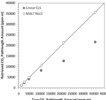
An alternative to CLS-based methods is to use a nonlinear least squares (NLLS) fitting procedure (Marquardt, 1963). This approach can fit single-beam spectra directly and re-quires no assumption of Beer-Lambert linearity, allowing for the use of both weak and strong absorption regions (Griffith et al., 2003). In a comparison between retrievals made using CLS and NLLS methods, Childers et al. (2002) found that for CO2, CH4, NH3and N2O, the CLS method generally
under-estimated at higher gas concentrations. To demonstrate this effect, Fig. 1 illustrates retrievals made here using the CLS and NLLS approach from spectra of a gas cell containing CO2gas of varying concentrations, topped up with nitrogen
to maintain ambient pressure (the experimental method is de-scribed fully in Sect. 3 of this paper). The underestimation of high CO2concentrations when using the CLS method is
clearly evident, and is due to the aforementioned nonlinear deviation from the Beer-Lambert law.
For volcanological applications, Horrocks et al. (2001) used a similar experimental setup and spectral modelling ap-proach to that employed here to test the accuracy of OP-FTIR retrievals of SO2 over a wide range of absorber amounts
(125 ppmm–10 500 ppmm). As is the case here, instead of using a White cell to increase pathlength, Horrocks et al. (2001) chose to use higher mixing ratios (ppm) of SO2,
which are equivalent to a longer path according to the Beer-Lambert law:
τ = α Lc (1)
where optical depth (τ, unitless) is equal to the product of the absorption coefficient of the sample (α, [ppmm]−1), the path length of the sample (L, m) and the mixing ratio of the sam-ple (c, ppm). Optical depth is related to the true transmission (T, unitless) following Eq. (2):
T = e−τ (2)
The measured transmittance is the true transmittance con-volved with the instrument line shape (ILS). Horrocks et al. (2001) found that increased retrieval accuracies were achieved as concentrations of SO2increased, improving from
∼5.6% at 125 ppmm to within 1.0% at 10 500 ppmm. This study builds on this work by using a similar approach to es-tablish the OP-FTIR retrieval accuracies for CO2, CO and
CH4 at mixing ratios ranging from those found in ambient
air to those found in polluted cities, biomass burning smoke
Fig. 1. Comparison of FTIR-derived retrievals of gas-cell CO2
pathlength amount to the true pathlength amount within the cell. Retrievals were made from the same spectra via two approaches, the Classical Least Squares (CLS) approach described in Haa-land (1990) and the MALT forward model and nonlinear least squares (NLLS) fitting procedure described in Griffith (1996) and Griffith et al. (2003). The 1:1 line is shown, and the increasing underestimation of the CLS-based retrievals at higher pathlength amounts is clearly evident.
and volcanic plumes, a much broader range than investigated by Esler et al. (2000). We follow Horrocks et al. (2001) and analyse the collected IR spectra using an iterative NLLS method coupled to a forward modelling approach, specif-ically the Multi-Atmospheric Layer Transmission (MALT) model described in Griffith (1996) and Griffith et al. (2003). The work of Lamp et al. (1997) showed how Beer-Lambert law divergence can impact retrieval accuracy when investi-gating high concentration gases using spectral regions con-taining strong IR absorbance features. Generating retrievals from modelled synthetic spectra fitted to the measured spec-tra in the way conducted here should avoid these problems and the associated concentration underestimation illustrated in the CLS-derived results displayed Fig. 1.
3 Instrumentation and setup
Table 1.Cell mixing ratios (ppm) and equivalent pathlength amounts (ppmm) for the 1.05 m gas cell filled with CO2, CH4and CO
respec-tively, with the equivalent mixing ratios for longer atmospheric paths (assuming the same temperature,∼20◦C, and pressure,∼1000 hPa
conditions) also given. For reference, ambient “clean” air mixing ratios of CO2, CH4and CO are circa 385 ppm, 1.8 ppm and 0.15 ppm,
respectively.
Cell mixing Cell Pathlength Equivalent Equivalent Equivalent
ratio amount mixing ratio for mixing ratio for mixing ratio for
(ppm) (ppmm) a 30 m path a 100 m path a 800 m path
(ppm) (ppm) (ppm)
CO2
12 014 12 612 420.4 126.1 15.8
24 991 26 236 874.5 262.4 32.8
45 799 48 080 1602.7 480.8 60.1
100 125 105 112 3503.7 1051.1 131.4
200 200 210 172 7005.7 2101.7 262.7
340 351 357 304 11910.1 3573.0 446.6
CH4
51.94 54.52 1.83 0.55 0.07
92.81 97.43 3.25 0.97 0.12
168.51 176.91 5.90 1.77 0.22
270.85 284.34 9.48 2.84 0.36
490.09 514.50 17.15 5.15 0.64
CO
18.96 19.90 0.66 0.20 0.03
244.14 256.30 8.54 2.56 0.32
459.13 482.00 16.07 4.82 0.60
1217.05 1277.67 42.59 12.78 1.60
6077.20 6379.91 212.66 63.80 7.98
Fig. 2.Schematic of the physical instrumentation arrangement used in the current study.
was a MIDAC Corporation FTIR Air Monitoring system, fit-ted with a mercury cadmium telluride (MCT) detector and ZnSe optics. The spectrometer was optically coupled to a 76 mm Newtonian telescope and placed to view an IR source through the IR transparent windows of the gas cell. The IR source used was a SiC globar operating at 1100 K, po-sitioned at the focus of a 150 mm collimator. This setup,
shown in Fig. 2, is very similar to that used by Horrocks et al. (2001), with a total pathlength of∼1.5 m, 0.5 m of which consisted of free air between the cell and spectrometer and cell and IR source, together with air inside the spectrome-ter housing. The CO2and H2O mixing ratios in the
the FTIR spectrometer telescope to avoid MCT detector sat-uration, and the temperature of the gas inside the gas cell measured using a platinum resistance thermometer (PRT).
Table 1 lists the gas mixtures investigated. As described by the Beer-Lambert law (Eq. 1), it is possible to simulate a longer OP measurement pathlength by increasing the mixing ratio of the gas sample inside the cell, since pathlength (L) and mixing ratio (c) equivalently increase the number of gas molecules in the open path over which the IR spectra are ac-quired. However, for target gas mixing ratios above∼1% (in air or N2) the linewidths will become significantly affected
by self broadening relative to longer path-lower concentra-tion spectra of the same total pathlength amount. This affects each of the CO2mixtures used in this study, but not the other
gases since their mixing ratios are significantly lower. The MALT model includes a mixing ratio-weighted linewidth to account for this self broadening effect.
The mixing ratios used here were chosen to represent a range covering those from clean air measured over short-to-long pathlengths in the natural environment (e.g. 10– 1000 m), as well as polluted air across the same pathlength range, and range up to mixing ratios that might be found in pollutant plumes (e.g. from industrial sources or biomass burning). For example, six different CO2
pathlength-concentration products (hereafter called pathlength amount) were used, spanning∼12 500 ppmm to∼360 000 ppmm. If these pathlength amounts are expressed as mixing ratios us-ing pathlengths typically employed in the field, both the low-est and highlow-est cell mixing ratios yield a CO2mixing ratio
of ∼420–450 ppm for a 30 m and 800 m path respectively, equivalent to typical ambient CO2conditions found in urban
settings (e.g. Rigby et al., 2008).
Gas mixtures were prepared manometrically using high purity (99.9%) component gases. The mixing method re-lied on three MKS Baratron (type 690) pressure capacitance manometers operated at three precision levels of 0.1 Pa, 10 Pa and 100 Pa with a stated accuracy of±0.05%. The manome-ters were also used to test the sealing of the gas cell, record-ing a<1% change in cell pressure over 18 h when filled to ambient pressure (1000 hPa). For each gas concentration to be studied, the cell was evacuated before the sample gas (CO2, CO or CH4) was slowly released into the cell until
the desired mixing ratio was reached. After waiting for the pressure to stabilise and noting the final pressure, the cell was filled with nitrogen to ambient pressure (1000 hPa) and allowed to stabilise once more. After stabilisation, 10 IR spectrum were measured with the FTIR spectrometer, each consisting of 8 co-added scans (a total of ∼9 s scan time per spectra) in order to increase signal-to-noise. The rela-tive standard deviations among each set of 10 replicate sin-gle beam spectral measurements ranged from 0.1–1.2%, with standard errors of the means of 0.03–0.4% for these measure-ment conditions. The partial pressure of the sample gas was used to calculate the true sample mixing ratio (ppm) by divid-ing the partial pressure of the sample gas by the final ambient
pressure of the gas cell. To avoid contamination by gas from the previous mixture, the lowest concentration of each gas was mixed first, working up to higher concentrations.
4 Procedure for gas concentration retrieval
4.1 Spectrum simulation and fitting algorithm
Spectra were analysed using a NLLS method combined with a forward modelling approach, whereby NLLS was used to fit a modelled spectrum to a measured spectrum, thus solving the inverse problem of returning gas concentrations from the observations. The method is quite commonly applied in OP-FTIR studies, and examples include SFIT2 (Rinsland et al., 1998), often used to retrieve total atmospheric column trace gas abundances (e.g. Hase et al., 2006; Fu et al., 2007 and Senten et al., 2008), but also used for ground-based open-path studies (e.g. Briz et al., 2007). A similar procedure (Bur-ton et al., 1998) has been commonly applied to the retrieval of gas concentrations from open path measurements of vol-canic plumes (e.g. Oppenheimer et al., 1998; Horrocks et al., 1999 and Richter et al., 2002). The specific retrieval pro-cedure used here is based on the Multi-Atmospheric Layer Transmission (MALT) model of Griffith (1996) and Griffith et al. (2003), whose past applications include the analysis of open-path, White cell, and solar occultation spectra (Goode et al., 1999; Goode et al., 2000; Bertschi et al., 2003; Galle et al., 2000; Griffith et al., 2002).
The background theory to the inverse problem is detailed in Rodgers (2000). By denoting the measurement spectrum as vectory(the measurement vector) and the variables to be retrieved (the trace gas concentrations) as the state vectorx, the measurement and its relation to the state vector, can be described as:
y = f (x) (3)
wheref (x) is the forward function, describing the physics of the measurement. It is unlikely that the physics of a sys-tem will be known and understood with full accuracy. Hence Eq. (3) is adapted as:
y =F (x) +ε (4)
F (x), the forward model, approximates the physics of the measurement, andε is the measurement error. HereF (x) represents the simulated single beam spectrum.
features within the spectral micro-window of interest. Calcu-lations are performed using the HITRAN database (Rothman et al., 2009), listing absorption line positions and strengths, widths and details of pressure and temperature dependencies for the given species.
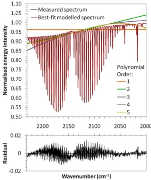
A polynomial function (the order of which is defined as a parameter by the user) is fitted to the measured spectrum and is used to simulate the 100% continuum line (i.e. the signal in the absence of the trace gas. Examples of different fit-ted polynomial functions are shown in Fig. 3. The forward model calculates the optical depth (OD) of the target gas at each wavenumberv as a function of the absorption coeffi-cient atvand the pathlength amount of each gas. A necessary parameter for this computation is the Voigt line shape – the convolution of the Doppler broadening Gaussian line shape function and the pressure broadening Lorentzian line shape function. The former is calculated using temperature and molecular weight, and the latter using the pressure depen-dence given in HITRAN. Convolving the line strengths from HITRAN with the line shape produces the absorption coeffi-cient used to calculate the optical depth. At wavenumberv, the overall OD is taken as the sum of all calculated ODs for all absorption lines for all species. The OD is then converted to a transmission measure and convolved with the instrument line shape (ILS) and the 100% continuum line to yield the final synthetic single-beam spectrum for the spectral window of choice (Fig. 3). The ILS is dependent on the apodization function used, the instrument field-of-view (FOV), and any modulation loss or phase error in the interferometer. These parameters can be retrieved during the NLLS fitting proce-dure.
The difference between the synthetic and measured spec-trum yields a residual specspec-trum (Fig. 3, bottom); and the chi-squared (χ2) statistic and the partial derivatives for each of the input parameters are calculated. The Levenburg-Marquardt method (Levenburg, 1944; Levenburg-Marquardt, 1963; Press et al., 1992) is used to find the least-squares linear best fit, and thus the set of optimum gas concentrations that min-imise the residual spectrum, based on pre-determined con-vergence criterion (χ2minimum).
4.2 Reported error
As with other spectrally-based retrieval approaches based on forward modelling and nonlinear fitting methods (e.g. Bur-ton, 1998), MALT reports the standard error for each of the retrieved trace gas amounts and the a priori input parame-ters (this metric is termed the reported error hereafter). For each iteration of the NLLS fitting procedure, the covariance matrix is determined from the standard deviation of the resid-ual spectrum (i.e. the synthetic spectrum subtracted from the measured spectrum). The reported error for parameterxi is
defined as the square root of the i-th diagonal element of the covariance matrix, and is influenced by choice of a priori fixed input parameters, model errors/lack of fit, measurement
Fig. 3.Examples of results from a measured spectrum and the best-fit modelled spectrum produced using the MALT forward model and nonlinear least squares (NLLS) fitting procedure described in Griffith (1996). The case shown is for 482 ppmm of CO at a gas pressure of 1000 hPa. Top: The measured and best-fit modelled spectra are shown to be well matched, with the different background polynomial functions (orders 1–5) tested also shown. The fourth or-der polynomial provided the best match to the measured spectrum, and this was used to simulate the best-fit modelled spectrum shown. Bottom: The residual spectrum (i.e. the measured spectrum sub-tracted from the modelled spectrum), which is used to provide a measure of fitting accuracy. The spectral features in the residual are due to an imperfect fit between the modelled ILS and the non-ideal instrument ILS.
noise, amount of information (the width of the spectral win-dow and intensity of signal within that winwin-dow) and degrees of freedom (which reduces with increasing number of param-eters).
5 Methodology
5.1 Determination of input parameters
When performing a spectral fit, the input parameters required by the spectral model (MALT) can be stated as fixed con-stants or can be included in the fitting process. These pa-rameters relate to the composition of the sample atmosphere (i.e. which gases are present in the sample and have absorp-tion lines in the spectral window of interest, the concentraabsorp-tion of these gases, and the temperature and pressure of the com-position) and to the instrument line shape (i.e. spectral shift, resolution, apodisation, FOV, phase and zero-line offset). In our experiment, whilst the gas concentration was fitted, the temperature and pressure of the sample were taken from the gas cell PRT and Baratron readings respectively. Determina-tion of instrument line shape parameters was, however, less straight forward:
– the spectral shift (correction for fractional wavenumber shifts in the position of absorption lines caused by inac-curate knowledge of the interferometer alignment) was fitted
– the spectral resolution was fixed at the manufacturer’s specification (0.5 cm−1)
– asymmetry in the line shape influenced by small changes in spectrometer alignment was also fitted through a variable phase error
– the field-of-view (determined by the spectrometer’s lim-iting aperture and collimator focal length) was ini-tialised at the manufacturer’s specification and fitted as described below to determine the effective value. Horrocks et al. (2001) demonstrate that their MIDAC spec-trometer’s effective field-of-view of 52 mrad differed signifi-cantly from the nominally quoted 20 mrad. We followed the methodology of Horrocks et al. (2001) to determine the field-of-view of the instrument used here, measuring the spec-trum of CO gas with narrow absorption lines at low pressure (401 hPa) so that the resulting measurement is primarily a function of the absorption feature convolved with the instru-ment line shape. 80 scans were co-added to create one par-ticularly low-noise spectrum. A series of MALT retrievals were run for a single absorption line at 2082 cm−1, and the
field-of-view parameter optimised to give the lowest reported error, whilst all other parameters remained fixed. The FOV parameter yielding the smallest reported error for the low-pressure CO absorption line was used as a fixed input for all other retrievals conducted here. Sensitivity to this param-eter was also investigated (see Sect. 5.3).To dparam-etermine the retrieval error of the reported concentrations, it is necessary to compare the retrieved concentrations with the true con-centration (i.e. to the cell concon-centrations listed in Table 1).
Retrieval error is therefore here defined as the true concen-tration subtracted from the reported concenconcen-tration, divided by the true concentration and expressed as a percentage.
One further consideration for the retrieval procedure is to account for any zero-baseline spectral offset that may result from photometric errors associated with the use of an MCT detector (M¨uller et al., 1999). Two factors might lead to a non-zero signal in spectral regions that should otherwise ex-hibit complete absorption. The first is caused by scattering of radiation that has not originated from the lamp source, po-tentially related to imperfections in instrument optics, such as dirty mirrors. This is a common occurrence in well used field spectrometers, particularly when deployed to dusty or corrosive environments. Furthermore, if the gas cell was at a different temperature to that of the interferometer, an ef-fect will appear in the measured spectrum. Whilst laboratory spectrometers often solve this problem by placing the inter-ferometer before the sample cell, this is not of the case for bistatic OP-FTIR field configurations (M¨uller et al., 1999). Neither the temperature of the gas cell nor spectrometer were controlled in this experiment, but were rather left to equili-brate to ambient temperature, and therefore small differences in temperature may have influenced the recorded spectra. The second factor which might lead to a non-zero baseline is detector saturation. MCT detectors saturate rather easily (Smith, 1995), and whilst efforts were made in this study to prevent detector saturation via use of the attenuator, some detector saturation effect may be present. Any zero-baseline offset caused by stray light or detector saturation will be ap-parent in spectral regions where the examined gases should absorb all incoming radiation (e.g. the CO2saturation band
at∼2350 cm−1). If an offset was present, this amount was subtracted from the spectrum before quantitative analysis.
5.2 Spectral window and “background” polynomial
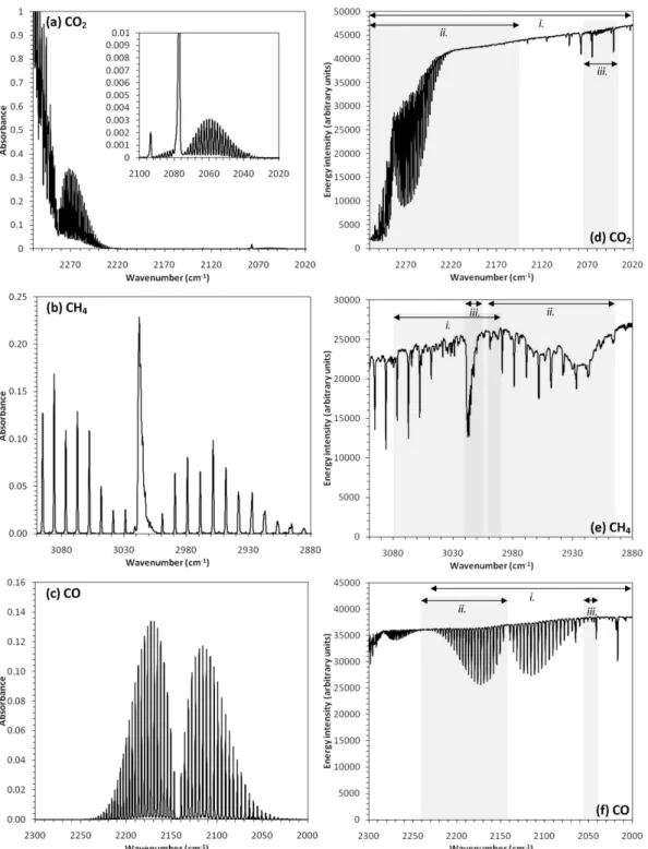
Fig. 4.Modelled and measured spectra at 0.5 cm−1wavenumber resolution for the CO2, CH4, and CO trace gases considered here. (left)
Absorbance spectra modelled using the MALT forward model; (right) Measured FTIR single-beam spectra. The various spectral windows
used to retrieve the trace gas concentrations from the measured spectra are indicated by the numbered horizontal arrows in(d),(e),(f)and
are detailed in Table 2.
by these, except perhaps across the narrow CH4spectral
win-dow.
For CO2(Fig. 4a and d), the widest spectral spectral
win-dow used here, 2020–2310 cm−1 (taken from Esler et al., 2000) was split into two sub windows, 2150–2310 cm−1
(location of primary absorption features of 13CO2 and 12CO
2) and 2034–2075 cm−1(location of the weaker12CO2
feature, see inset in Fig. 4a). For each window, CO2retrievals
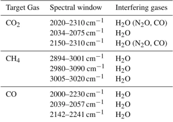
Table 2.Spectral windows used here for the retrieval of CO2, CH4
and CO and marked in Fig. 4. Also listed are the potentially interfer-ing gases (those in brackets were not included in the forward-model spectral simulation conducted here due to the very short clean air atmosphere path used, but would generally be required over longer pathlengths in the ambient atmosphere).
Target Gas Spectral window Interfering gases
CO2 2020–2310 cm−1 H2O (N2O, CO)
2034–2075 cm−1 H2O
2150–2310 cm−1 H2O (N2O, CO)
CH4 2894–3001 cm−1 H2O
2980–3090 cm−1 H2O
3005–3020 cm−1 H2O
CO 2000–2230 cm−1 H2O
2039–2057 cm−1 H2O
2142–2241 cm−1 H2O
vapour was certainly present in the ambient part of the path external to the gas cell and has absorption lines in these spec-tral windows, H2O was also included in the retrievals. Whilst
CO and N2O also absorb within these spectral windows, they
were not present in sufficient amounts to be significant. In field situations using longer pathlengths, CO and N2O may
affect the measured signal and should therefore be included in any retrieval procedure. For CH4, Esler et al. (2000) use a
broad spectral window, 2810–3150 cm−1. Unfortunately, the
majority of this window is affected by a spectrometer arte-fact (2800–2990 cm−1, see Fig. 4b and e), believed to be
caused by residue on the instrument optics. The complex-ity introduced by the artefact significantly hinders the abil-ity to model the spectrum using a lower-order (<6) polyno-mial. Two spectral windows were therefore selected so as to exclude the effects of this artefact, a broad window (2980– 3090 cm−1), that maximises the number of CH4absorption
lines, and a narrower window concentrating on the strongest lines (3005–3020 cm−1). In addition, a third window, lying within the region where lines are affected by the detector artefact (2894–3001 cm−1) was also investigated. For CO (Fig. 4c and f), Esler et al. (2000) use a broad window en-compassing the entire CO absorption feature and a similar window is used here (2000–2230 cm−1). In addition, two
narrower windows, one featuring only one branch of the CO absorption feature (2142–2241 cm−1) and the other
featur-ing only four weaker CO absorption lines (2039–2075 cm−1) were also investigated.
5.3 Sensitivity analysis and error budget
A local sensitivity analysis was performed in order to de-termine the influence of model parameter uncertainty on
retrieval accuracy. Uncertainties in temperature, pressure and spectrometer FOV were considered, which may result from field situations where the measurement conditions are less tightly controlled than is possible in the laboratory. In particular, it can be difficult to measure temperature and pressure precisely in some open-path geometries, particu-larly when analysing high altitude plumes, or ones where the plume is generated by high temperature volcanological or combustion-related processes. Pressure and temperature are important in the retrieval procedure as they affect the shape of gas absorption features upon which the fit between the measured and modelled spectra depends. Assumed pressure determines the Lorentzian line shape of absorption lines in the simulated spectra. Higher pressures lead to a broadening of line widths, and the maximum line depth is suppressed. Whilst the relatively low (0.5 cm−1) spectral resolution of the
FTIR spectrometer used here is responsible for the majority of observed linewidths, this pressure-related broadening does also influence the retrieval process. Pressure broadening for any sample gas is also related to the other gases contained in the gas mixture.
The influence of assumed temperature is to affect the strengths of individual absorption lines and the band shape of the modelled spectra. Doppler broadening caused by the temperature-dependent distribution of molecular velocities within gases (as well as a minor influence on line broad-ening) contributes to the temperature dependence of line-shapes. The primary influence of temperature and pres-sure, however, is in the calculation of the mixing ratio from the retrieved number of gas molecules per square cm (molecules cm−2) output from the retrieval process (the
ab-sorption features present in the spectra are a direct function of the number of molecules of the target gas in the opti-cal path). The relationship between the concentration of a particular gas in a sample, in molecules per square centime-tre (X, molecules cm−2) and the mixing ratio of the gas (x, ppm), pressure (p, hPa), temperature (T, K) and pathlength of the sample (L, m) is described in Eq. (5), whereAis Avo-gadro’s constant (6.022×10²³mol−1) andRis the gas con-stant (8.314 J [mol K]−1):
X = xLpA
RT (5)
Any error in assumed pressure or temperature will there-fore cause a proportional error in retrieved mixing ratio (x) through Eq. (5); whereas, retrievals in molecules cm−2will
only be affected by the influence of pressure and temperature errors on the modelled spectra. In many applications, OP-FTIR is used to investigate concentration ratios of two gases, for example CO2:CO in biomass burning studies (Yokelson
et al., 1997) or SO2:HCl in volcanological applications
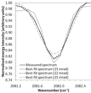
Fig. 5.Sensitivity of the reported error (based on the fit residuals) and retrieval error (based on the difference between retrieved path-length trace gas amount and actual pathpath-length trace gas amount) to assumed instrument FOV. The example is shown for CO trace gas
retrievals based on the CO absorption line centred at 2082 cm−1
(Fig. 6). Measurements were made at a low pressure of 400.5 hPa with a true CO mixing ratio of 1217.05 ppm. Reported error is min-imised at an assumed FOV of 22 mrad, though is relatively insen-sitve to the FOV variations studied here. Retrieval error is, however significantly more sensitive, and assumed 20 mrad FOV yields the smallest actual retrieval error.
here, pressure and temperature-independent amounts (in molecules cm−2) were used for the comparison. Pressure and temperature inputs were varied systematically by up to ±20◦C and ±200 hPa respectively; ranges that might be found over altitude differences of up to 3 km. Retrieved con-centrations were compared with true concon-centrations to yield both the retrieval error and sensitivity to the pressure and temperature assumptions.
6 Results and discussion
6.1 FOV determination
Figure 5 shows how the reported error (i.e. the MALT fitting error, quantified as a percentage of the retrieved concentra-tion in Sect. 4.2) and the actual retrieval error (quantified as the percentage difference between the retrieved gas concen-tration and the true gas concenconcen-tration in Sect. 4.2) varies with assumed field-of-view. Actual retrieval error is much more sensitive to FOV variations than is the reported error. The lowest reported error occurs at a FOV of 22 mrad, whereas the lowest retrieval error occurs at a FOV of 20 mrad. As-sumed FOV significantly larger or smaller than the 22 mrad optimum value resulted in increasingly poor fits between the modelled and measured CO spectrum (Fig. 6). Unlike Hor-rocks et al. (2001), we found the optimal FOV, according to
Fig. 6.Measured single-beam spectra and best-fit modelled spectra
for the CO absorption line centred at 2082 cm−1at a gas pressure
of 400.5 hPa. Modelled spectra were simulated assuming different fields-of-view (15–25 mrad), with the 22 mrad FOV providing the best match between the measured and modelled spectra.
the reported error, to be similar to the nominal FOV stated by the instrument manufacturer, and we attribute the 2 mrad (10%) discrepancy to off-axis rays caused by a combination of small misalignments of spectrometer and telescope optics, and an imperfect source collimator. Horrocks et al. (2001) also found a discrepancy between the FOV parameter yield-ing the lowest reported error and those that yielded the low-est retrieval error. This discrepancy may be explained by our use of nitrogen as a buffer gas, given that line broad-ening coefficients in the HITRAN08 database (Rothman et al., 2009) relate to the gas of interest in air, and not when mixed with nitrogen. The difference between nitrogen and air broadening is of the order of∼10%. This factor, com-bined with uncertainties in HITRAN, or an inability of the forward modelling and NLLS fitting procedure to accurately retrieve concentrations using a single absorption line given the relatively low spectral resolution of the instrument, may also explain this discrepancy. By retrieving concentrations using broader spectral features, the retrieved effect of instru-ment line shape inaccuracies on individual absorption lines are decreased. The effects of degrading the assumed spec-tral resolution from the highest 0.5 cm−1value were
investi-gated, but increased the reported errors, and therefore further adjustments to this factor were not required.
6.2 Spectral window and background polynomial
6.2.1 Carbon dioxide
Fig. 7.Retrieval errors for CO2, CH4and CO trace gas retrievals resulting from use of the MALT model and NLLS fitting procedure with
OP-FTIR spectra from a gas cell containing samples of these three gases over wide concentration ranges. Retrievals were made using three different spectral windows for each trace gas and three different polynomial orders. In order to aid comparison of the error magnitudes for the retrievals of each trace gas, the same y-axis range is used to display the results from the three spectral windows tested. Retrieval error magnitude is seen to vary quite widely between the different spectral windows used to retrieve the pathlength amount of a particular trace gas, and for some windows between the different polynomial orders examined.
individual absorption lines (Fig. 4 and Table 2). For CO2,
results shown in Fig. 7 indicate that the absolute retrieval er-ror for 5 of the 6 pathlength amounts tested is at a minimum for the 2150-2310 cm−1 spectral window using a fourth-order polynomial, with retrieved pathlength amounts over the full range tested having a root mean squared (RMS) error of 2.4% (Fig. 7b). Whilst the results show little sensitivity to the use of a fourth or fifth-order polynomial, the use of a third-order polynomial leads to a noticeable increase in re-trieval error. A third-order polynomial is insufficient to de-scribe the background shape of a spectral window as wide as 2150–2310 cm−1. Moreover, the background shape of this window is complicated by the CO2absorption feature that
strengthens to saturation at 2310 cm−1(Fig. 4a). Retrieval errors are highest for the broader, 2020–2310 cm−1 spec-tral window (Fig. 7a), though the reported error (not shown)
is lowest for this window (0.1%, compared with 0.3% for 2150–2310 cm−1and 0.9% for 2034–2075 cm−1). This ap-parent contradiction may be explained by the presence of a large featureless baseline across most of this wider spectral window (Fig. 4a) leading to an overall improved fit between the modelled and measured spectrum, though not necessar-ily the best fit at the wavenumber location of the absorption features. A wider spectral window typically decreases the ability of any particular polynomial to model the background continuum as is the case here. There is also an additional rea-son why use of the broader spectral window generally leads to greater inaccuracy. This is because the zero-baseline off-set can only be calculated from data collected in the CO2
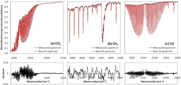
Fig. 8.Examples of measured spectra and best-fit modelled spectra made using the optimum spectral windows and a fourth-order polynomial
background (top), and the residual between the measured and modelled spectra (bottom) for(a)CO2;(b)CH4; and(c)CO. Modelled spectra
were simulated using MALT and the best-fit modelled spectra were found using the NLLS fitting procedure.
spectral window (2034–2075 cm−1) used here for CO2
re-trieval are less influenced by the choice of polynomial order, each having RMS errors of less than 3.7% (Fig. 7c). The flatter background continuum in this window, combined with the presence of fine absorption structure in the CO2lines,
ex-plains the reduced sensitivity to polynomial order. The inac-curacy of the retrievals made at lower pathlength amounts in this spectral window is most likely due to the weaker nature of the absorption lines at 2034–2075 cm−1.
Our results clearly indicate that the choice of spectral win-dow, coupled with an appropriate choice of background poly-nomial, have a strong influence on CO2 retrieval accuracy.
Broader windows typically contain more information, poten-tially improving the fit between the modelled and measured spectra. However, it is also important to ensure that the back-ground continuum of the spectrum within the window under study can be sufficiently well represented by the chosen poly-nomial. Our results suggest that whilst the 2020–2310 cm−1 spectral window used for CO2retrieval gives the lowest
re-ported errors (based on the fit residuals; Sect. 4.2), it does not result in the lowest retrieval error. The 2150–2310 cm−1 spectral window, used with a fourth-order polynomial actu-ally provides the lowest retrieval error for CO2, ranging from
−1.9% to 4.3% across all pathlength amounts tested. An ex-ample spectrum with best-fit modelled spectrum is shown in Fig. 8a.
6.2.2 Methane
As outlined in Sect. 5.2, retrievals of CH4were confounded
by an instrument artefact in the relevant absorption region. The spectral window tested that covered this region (2894– 3001 cm−1) showed both large reported and retrieval errors,
regardless of the polynomial order chosen (Fig. 7e). The lowest retrieval errors for CH4come instead from the 2980–
3090 cm−1spectral window that excludes the artefact region (Fig. 7d), with a fourth-order polynomial yielding an RMS error of 1.4% (Fig. 8b shows an example spectrum with a best-fit modelled spectrum for this spectral window). As was the case with the narrowest (2034–2075 cm−1) CO
2
re-trieval window, the polynomial order does not significantly influence retrieval accuracy due to the fine structure of the CH4 absorption lines and the flat background continuum.
However, for the narrowest CH4 retrieval window tested
(3005–3020 cm−1), the polynomial order has a strong in-fluence (Fig. 7f) with only a first order function allowing pathlength amounts to be retrieved within an RMS error of 3.9%. Individual CH4absorption lines remain unresolved at
the 0.5 cm−1spectral resolution used here, and instead com-bine to appear as one large apparent absorption feature, and thus higher order polynomials incorrectly start to fit this fea-ture as well as the background continuum.
6.2.3 Carbon monoxide
Results for CO suggest that the two broadest spectral win-dows provide very similar retrieval accuracies (Fig. 7g and h), with the 2000–2230 cm−1spectral window used with
windows tested here showed a lower reliance on choice of background polynomial compared to the other gases, reflect-ing the “flat” background continuum across the whole CO absorption feature (Fig. 4f). Results from the narrower 2039– 2057 cm−1spectral window indicate that it is best suited to retrieval of higher pathlength amounts (Fig. 7i), with poor re-trieval accuracies for pathlength amounts below 1000 ppmm. High reported errors (based on the fit residuals) suggest that the retrieval process performs poorly with the weak absorp-tion lines in this spectral window, as is also the case for lower pathlength amounts of CO2retrieved in the 2034–2075 cm−1
spectral window.
6.3 Sensitivity analysis and error budget
Using the optimum set of retrieval parameters described in Sect. 6.2, a series of sensitivity analyses were performed. In Sect. 6.1, the spectrometer FOV was determined as 22 mrad. The exact FOV is difficult to determine given the fast optics and the absence of a well defined limiting aperture. We com-pared retrievals made using our optimally determined FOV with those made using a FOV varied by±10%.
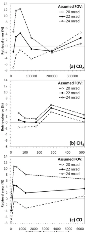
Retrievals for all three gases generally show a system-atic reliance upon the specified FOV (Fig. 9), with re-trieved pathlength amounts generally increasing with as-sumed FOV. CO demonstrated the greatest sensitivity to FOV since the CO absorption lines are narrower than the instru-ment’s 0.5 cm−1spectral resolution and their representation is therefore strongly influenced by instrument parameters. CO2 retrieval accuracy appears to be less sensitive to FOV
uncertainty at higher pathlength amounts. This may be ex-plained by the increasing saturation (absorption of all source energy) by strong absorption lines at higher CO2pathlength
amounts, leaving fewer lines in the spectral window affected by errors in FOV.
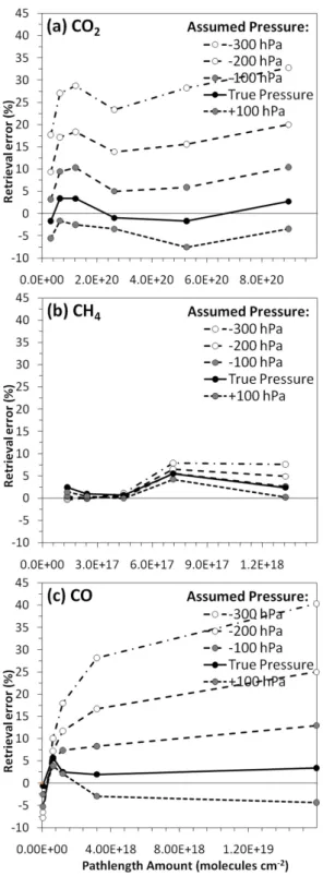
The retrieval sensitivities to assumed pressure and temper-ature were calculated from the pressure- and tempertemper-ature- temperature-independent molecular amounts (molecules cm−2), rather than from the volumetric mixing ratios (ppmm), as the lat-ter are additionally sensitive to these paramelat-ters via the re-lationship used to interconvert between these two concentra-tion units (Eq. 5). Figure 10 shows the sensitivity of the re-trievals to assumed gas pressure, where it can be seen that pathlength amounts are generally overestimated when pres-sure is underestimated, and vice versa. As is the case with the FOV parameter, the modelled absorption line widths are affected by the assumed pressure (Fig. 11a and b). When a lower pressure is assumed, narrower lines than are actu-ally present in the measured spectrum are modelled due to inadequate pressure broadening, causing a positive residual between the modelled spectrum and the measurement (sim-ilar to the residual spectrum in Fig. 11b. In order to fit the modelled spectrum to the measured spectrum, the NLLS pro-cedure increases the concentration of the absorber to min-imise this positive residual, leading to an overestimation of
Fig. 9. Sensitivity of trace gas concentration retrieval error to the
assumed FOV for(a)CO2,(b)CH4, and(c)CO. Retrievals were
Fig. 10. Sensitivity of trace gas concentration retrieval error to the
assumed gas pressure for(a)CO2,(b)CH4, and(c)CO. Retrievals
were made using the MALT model with a NLLS fitting procedure. The same y-axis range is used in each case to aid comparison of error magnitude between gases.
gas pathlength amounts, whereas the reverse is true when as-sumed pressure is overestimated.
For CH4and lower pathlength amounts of CO, the error
in-duced by pressure uncertainties was significantly lower than for CO2(Fig. 10). As pathlength amounts increase,
absorp-tion lines deepen, causing any line shape inaccuracies due to incorrect pressure specification to be exacerbated. For CO2, line deepening is less of an issue, given that deep
ab-sorption lines occur for all pathlength amounts in the spec-tral window chosen, and this explains why CO2 retrievals
shows a higher sensitivity to pressure uncertainties at all pathlength amounts, with the percentage error relatively in-dependent of actual concentration. We find that the reported errors based on the modelled fit residuals show little depen-dence on pressure (±0.04%, ±0.01% and±0.002% across ±100 hPa for CO2, CH4 and CO respectively), whereas
re-trieval errors show a much greater sensitivity. In field sit-uations, pressure uncertainties are most likely to arise from uncertainty in plume height. Our analysis shows that uncer-tainties of up to 500 m at sea level (∼50 hPa) are therefore equivalent to a±0.5% uncertainty in CH4and low CO path-length amounts, but are closer to±3% for CO2 and higher pathlength amounts of CO.
Figure 12 shows the sensitivity of retrieved pathlength amount to assumed temperature. For CH4 and CO
re-trievals, temperature increases lead to proportional in-creases in retrieved pathlength amounts, whilst for CO2,
this effect is not observed at lower pathlength amounts and is reversed for the highest pathlength amounts (above 5×10²⁰molecules cm−2). These findings are best explained
by the temperature dependence of spectral band shape. Changing temperature affects the envelope of the absorption band (Fig. 11c), with higher temperatures causing more ab-sorption in the weaker lines that lie towards the edge of the band, and reduced absorption in the stronger lines located towards the middle of the band. Therefore, for spectral win-dows containing strong absorption lines located towards the middle of an absorption band, when assumed temperature is overestimated, a higher gas concentration is required for the modelled spectrum to best-fit the measured spectrum. When a spectral window containing weaker absorption lines at the edge of an absorption band is used, the opposite is true. For the CH4 and CO spectral windows, these effects
largely cancel each other out as the spectral windows lie across both strong and weaker lines at the middle and edge of their respective absorption bands. The greater influence of the stronger absorption lines leads to a small positive sen-sitivity for CH4and CO in the spectral windows used here.
For CO2, however, the saturation of the strongest lines
Fig. 11. Simulated transmission spectra for CO gas at a fixed molecular amount of 6.424×10¹⁷molecules cm−2, along with percentage
difference in transmission between the CO transmission spectra simulated using(a)an assumed FOV of 15 mrad and 25 mrad;(b)at 600 and
1200 hPa; and(c)at 270 K and 330 K. The figure focuses on thep-branch of the CO vibrational stretching mode absorption feature, centred
at 2143 cm−1. Increasing FOV leads to broader, but weaker absorption lines; increasing pressure leads to deeper and broader absorption
lines; whilst increases in temperature lead to stronger absorption towards the edge of the band (wavenumbers<2100 cm−1)and weaker
absorption towards the band centre (wavenumbers>2100 cm−1).
6.4 Sensitivity summary
Table 3 summarises the findings of the sensitivity analyses and indicates to what percentage accuracy CO2, CH4and CO
can be retrieved assuming optimum parameterisation of the forward model. The “worst-case” scenario (as suggested by Horrocks et al., 2001) indicates that the total error due to un-certainties that could arise from incorrect retrieval parame-terisation amounts to less than 8.2% for all tested pathlength amounts, with a mean of 4.8%. Generally these “external” errors are of a similar magnitude to the additional errors that maybe introduced via the uncertainty inherent in the absorp-tion line intensities for each gas. The HITRAN08 absorpabsorp-tion line intensity uncertainties are reported to be between 5–10% for CO2and CH4, but are lower for CO at 1–2% (Rothman
et al., 2009). Of course, with good meteorological measure-ments and careful collection of non-saturated single-beam spectra, the magnitude of the external errors can be min-imised. Whilst a global/variance-based sensitivity analysis may theoretically offer the potential to provide further in-formation about the effects of simultaneous uncertainties in multiple inputs (e.g. Petropoulos et al., 2009), the linear sen-sitivity of the output gas amounts to uncertainties in the three input parameters suggests that the local sensitivity analysis performed here is perfectly adequate for our purposes.
Errors in assumed pressure become increasingly signifi-cant at higher pathlength amounts, due to the deepening of absorption lines, especially for CO2 and CO. One solution
to this problem would be to use a spectral window with weaker absorption lines; however, the results for tempera-ture sensitivities indicate that this would increase sensitivity to the spectral band shape dependence on temperature. Er-rors in assumed temperature of less than 10◦C lead to er-rors in retrieved concentration of below 3%. Greater erer-rors are perhaps most likely to occur during studies focused on
plumes from hot sources (volcanic, fire or industrial), and care should be taken to minimise sensitivity to these errors by using a broad spectral window encompassing weak and strong absorption lines and ideally targeting plumes once they have cooled to near ambient temperatures at some dis-tance from the source region.
In our experiment, the spectrometer FOV was determined to be 10% higher than the manufacturer’s nominal value of 20 mrad. Unlike gases such as SO2, ambient and elevated
pathlength amounts of CO2, CH4and CO demonstrate deep
absorption lines that increase their sensitivity to instrument line shape, and therefore extra care should be taken to pre-serve instrument optics from degradation if measurements are to target these gases.
7 Summary and implications for field measurements
We investigated the accuracy of trace gas retrievals made us-ing a field-portable FTIR spectrometer under conditions that replicated those likely to be encountered in many field sit-uations, e.g. uncertain gas temperature, pressure and instru-ment line shape/FOV characteristics, and attempted to de-termine the optimum spectral window within which the re-trieval should be made under different measurement condi-tions. Our study was based on the measurement of gases contained within a 1 m gas cell, from which we collected 0.5 cm−1wavenumber resolution single-beam IR spectra of
CO2, CH4 and CO over a very broad range of pathlength
amounts, representing equivalent mixing ratios from those found in the clean, ambient atmosphere to the highly pol-luted plumes of biomass burning, volcanoes and industry over pathlengths of tens to hundreds of metres (Table 1).
Fig. 12. Sensitivity of trace gas concentration retrieval error to the
assumed gas temperature for(a)CO2, (b)CH4, and(c)CO.
Re-trievals were made using the MALT model with a NLLS fitting pro-cedure. The same y-axis range is used in each case to aid compari-son of error magnitude between gases.
Fig. 13.Relationship between mean retrieved pathlength trace gas amounts made using the optimum parameterisation of the MALT model determined herein. The 1:1 line is shown and all retrieved amounts are within 4.8% of true amounts (note logarithmic axes).
and those that maximised the amount of absorption informa-tion for each gas (e.g. the number of absorpinforma-tion lines) typi-cally produced the lowest reported errors (model fit residu-als) and the lowest actual retrieval errors when compared to the true gas cell pathlength amount. However, if broad spec-tral windows are to be used it is important to ensure a good background polynomial fit in the model (which is used to represent the continuum radiation), and we found that when wider windows were investigated, containing large regions showing no absorption (e.g. 2020–2310 cm−1for CO2),
re-trieval accuracies were degraded due to poor background fit-ting. Similarly, it is important to check that broader win-dows do not contain spectral artefacts, such as those found here in the 2894–3001 cm−1spectral window when
retriev-ing CH4. Such artefacts, potentially caused by contaminating
substances on the spectrometer optics, will complicate the simulation of the continuum background shape using lower-order polynomials, and should be carefully avoided.
When using the optimum parameterisation of the MALT forward model and nonlinear least squares fitting procedure deployed in the retrievals made here, we were able to retrieve trace gas pathlength amounts to within 4.8% of the true val-ues for all gases and pathlength amounts tested (Fig. 13). Mean retrieval errors were 2.4%, 1.4% and 3.6% for CO2,
CH4 and CO, respectively. A series of analyses was
Table 3.Summary of errors associated with parameter uncertainty when retrieving trace gas amounts from OP-FTIR measurements using the MALT foward model of Griffith (1996) with a NLLS fitting procedure. Errors for choice of polynomial and errors in assumed field-of-view, pressure and temperature are taken from the results presented in Figs. 7, 9, 10 and 11, and are calculated using the difference between the retrievals made using the best parameter to those using the altered parameter, expressed as a percentage. For example, at an actual
CO2pathlength amount of 12 612 ppmm, the retrieved CO2column amount based on the retrieval method parameterised with the optimum
parameter values was underestimated by just under 2%. Uncertainties in the HITRAN08 database (Rothman et al., 2009) refer to the line intensity error specified therein.
Retrieval Error (%), for CO2pathlength amounts (ppmm):
Source of Error 12 612 26 235 48 080 105 112 210 172 357 304
Choice of polynomial (4th or 5th order) 0.9 0.6 1.7 1.8 1.5 0.9
Field-of-view (best-fit or manufacturer’s) 5.2 6.2 5.5 3.2 0.2 1.8
50 hPa error in assumed pressure 2.2 2.8 3.2 2.1 3.4 3.5
10◦C error in assumed temperature 4.2 4.5 1.0 2.5 0.6 4.3
Total (added in quadrature) 7.1 8.2 6.7 4.9 3.8 5.9
Uncertainty in line intensities (HITRAN08) 5.0–10.0 5.0–10.0 5.0–10.0 5.0–10.0 5.0–10.0 5.0–10.0
Mean reported error 0.2 0.3 0.4 0.4 0.3 0.3
Optimum retrieval model parameters −1.9 3.1 4.3 −1.0 −1.7 2.7
Retrieval Error (%), for CH4pathlength amounts (ppmm):
54.5 97.4 176.9 284.3 514.5
Choice of polynomial (4th or 5th order) 1.6 0.8 0.6 0.7 1.0
Field-of-view (best-fit or manufacturer’s) 2.4 1.6 1.4 1.3 1.2
50 hPa error in assumed pressure 0.8 0.4 0.3 0.3 0.6
10◦C error in assumed temperature 2.8 2.2 2.1 1.9 1.5
Total (added in quadrature) 4.1 2.9 2.6 2.4 2.2
Uncertainty in line intensities (HITRAN08) 5.0–10.0 5.0–10.0 5.0–10.0 5.0–10.0 5.0–10.0
Mean reported error 2.0 0.9 0.6 0.6 0.8
Optimum retrieval model parameters 0.8 0.2 0.1 4.8 1.3
Retrieval Error (%), for CO pathlength amounts (ppmm):
19.9 256.3 482.0 1,277.7 6,379.9
Choice of polynomial (4th or 5th order) 0.2 0.0 0.0 0.0 0.0
Field-of-view (best-fit or manufacturer’s) 4.0 5.4 5.4 5.1 2.4
50 hPa error in assumed pressure 1.7 0.5 1.3 2.8 4.3
10◦C error in assumed temperature 0.2 0.8 0.9 1.0 1.0
Total (added in quadrature) 4.4 5.5 5.6 5.9 5.0
Uncertainty in line intensities (HITRAN08) 1.0–2.0 1.0–2.0 1.0–2.0 1.0–2.0 1.0–2.0
Mean reported error 0.5 0.1 0.1 0.1 0.1
Optimum retrieval model parameters −4.0 4.4 4.3 2.0 3.4
dependent on the assumed instrument FOV, due to the partic-ular narrowness of the CO absorption lines which remain un-resolved at the 0.5 cm−1resolution used here. The sensitivity
of all retrievals to FOV increased when the spectral window used for the analysis contained strong absorption lines, which occurred at higher pathlength amounts for the CH4and CO
spectral windows, but at lower pathlength amounts for the CO2spectral window (where higher pathlength amounts led
to absorption saturation, and therefore, a smaller number of observed absorption lines).
Generally, our results indicate that reported errors, which are based on the residuals between the best-fit forward mod-elled spectra and the measured spectra, are smaller than the actual retrieval errors and do not always vary in the same
concentration retrieval, given that errors induced by one pa-rameter may be compensated for by adjusting the value of another parameter to minimise reported error, but that this may result in an incorrect retrieval.
We found that retrieval sensitivity to uncertainties in tem-perature and pressure were relatively small for the magni-tude of parameter uncertainty that might be expected in typ-ical field situations. Assuming a potentially “worst-case” scenario of a 50 hPa and 10◦C error in assumed pressure and temperature, and the 10% difference in FOV found here as compared to the instrument manufacturer’s specification, pathlength amount retrievals might vary by up to 8.2% (er-rors added in quadrature). As discussed by Horrocks et al. (2001), gases that demonstrate individual absorption lines that are resolved in the spectra (as opposed to gases such as SO2, which has broad bands for which individual rotational
lines cannot be resolved), are more susceptible to parameter errors affecting spectral line shape. Minimising uncertainty in these parameters is therefore paramount for retrievals of CO2, CH4 and CO via a combination of accurate
temper-ature and pressure information, and careful examination of the spectral fit. In particular, as demonstrated in this study, errors due to poor zero-baseline offset correction, incorrect pressure, temperature, and instrument line shape assump-tions will all cause a poor fit when a retrieval is performed using a window containing both weak and strong absorption lines, and minimising reported errors in such a window will improve retrieval accuracy.
Our results confirm that a forward modelling approach coupled with a nonlinear least squares fitting routine can be a viable and accurate method for retrieving gas concentrations from OP-FTIR data, in this case using an MCT detector cov-ering a wide spectral range (600–6000 cm−1). Whilst it re-mains difficult to use the reported errors (model fit residuals) to provide a quantitative measure of actual concentration re-trieval error, our results provide confidence that carefully un-dertaken retrievals made using the forward modelling NLLS method deployed here can indeed provide good retrieval ac-curacies in the types of field situation where OP-FTIR could be very usefully deployed. Using an optimum parameterisa-tion of the model, we were able to retrieve the concentraparameterisa-tions of the three most abundant carbonaceous gases in the atmo-sphere to better than 5% over a very wide range of pathlength amounts (Fig. 13).
Acknowledgements. We would like to thank NERC MSF and their staff at RAL, particularly Robert McPheat and Kevin Smith, for their invaluable contribution to the experimental component of this work, and Christopher MacLellan and Alasdair MacArthur of NERC FSF for their wide ranging support, including loan of the FTIR spectrometer used here. We are very grateful for the expertise provided by Peter Zemek and Don Mullally (MIDAC Corporation), Clive Oppenheimer (University of Cambridge) and Mike Burton (Istituto Nazionale di Geofisica e Vulcanologia) at various points during the study, including during parts of the measurement campaign. Funding for the studentship of T. E. L. Smith comes
from NERC/ESRC Studentship ES/F012551/1. The contribution of Martin Wooster was supported by the NERC National Center for Earth Observation (NCEO).
Edited by: D. Feist
References
Bacsik, Z., Mink, J., and Keresztury, G.: FTIR spectroscopy of the atmosphere I. Principles and methods, Appl. Spectrosc. Rev., 39, 295–363, 2004.
Bertschi, I., Yokelson, R. J., Ward, D. E., Babbitt, R. E.,
Su-sott, R. A., Goode, J. G., and Min Hao, W.: Trace gas
and particle emissions from fires in large diameter and be-lowground biomass fuels, J. Geophys. Res., 108(D13), 8472, doi:10.1029/2002JD002100, 2003.
Briz, S., de Castro, A. J., D´ıez, S., L´opez, F., and Schafer, K.: Remote sensing by open-path FTIR spectroscopy, Comparison of different analysis techniques applied to ozone and carbon monoxide detection, J. Quant. Spectrosc. Ra., 103, 314–330, 2007.
Burton, M. R.: Remote sensing of the atmosphere using Fourier transform spectroscopy, PhD thesis, Department of Chemistry, University of Cambridge, 1998.
Burton, M. R., Allard, P., Mure, F., and La Spina, A.: Magmatic gas composition reveals the source depth of slug-driven strombolian explosive activity, Science, 317, 227–230, 2007.
Childers, J. W., Thompson Jr., E. L., Harris, D. B., Kirchgess-ner, D. A., Clayton, M., Natschke, D. F., and Phillips, W. J.: Multi-pollutant concentration measurements around a concen-trated swine production facility using open-path FTIR spectrom-etry, Atmos. Environ., 35, 1923–1936, 2001.
Childers, J. W., Phillips, W. J., Thompson Jr., E. L., Harris, D. B., Kirchgessner, D. A., Natschke, D. F., and Clayton, M.: Compar-ison of an Innovative Nonlinear Algorithm to Classical Least-Squares for Analyzing Open-Path Fourier Transform Infrared Spectra Collected at a Concentrated Swine Production Facility, Appl. Spectrosc., 56(3), 325–336, 2002.
Esler, M. B., Griffith, D. W. T., Wilston, S. R., and Steele, L. P.: Precision trace gas analysis by FT-IR spectroscopy 1.
Simulta-neous analysis of CO2, CH4, N2O and CO in air, Anal. Chem.,
72(1), 206–215, 2000.
Fu, D., Walker, K. A., Sung, K., Boone, C. D., Soucy, M.-A., and Bernath, P. F.: The portable atmospheric research interferomet-ric spectrometer for the infrared, PARIS-IR, J. Quant. Spectrosc. Ra., 103, 362–370, 2007.
Galle, B., Bergquist, B., Ferm, M., T¨ornquist, K., Griffith, D. W. T., Jensen, N. O., and Hansen, F.: Measurement of ammonia emis-sions from spreading of manure using gradient FTIR techniques, Atmos. Environ., 34, 4907–4915, 2000.
Gerlach, T. M., McGee, K. A., Sutton, A. J., and Elias, T.: Rates
of volcanic CO2degassing from airborne determinations of SO2
emission rates and plume CO2/SO2: Test study at Pu’u “O”o