www.atmos-chem-phys.net/15/6503/2015/ doi:10.5194/acp-15-6503-2015
© Author(s) 2015. CC Attribution 3.0 License.
Particulate emissions from residential wood combustion in Europe –
revised estimates and an evaluation
H. A. C. Denier van der Gon1, R. Bergström2,3, C. Fountoukis4, C. Johansson5,6, S. N. Pandis4,7, D. Simpson8,9, and A. J. H. Visschedijk1
1TNO, Dept. of Climate, Air and Sustainability, Princetonlaan 6, 3584 CB Utrecht, the Netherlands 2Dept. Chemistry & Molecular Biology, University of Gothenburg, 41296 Gothenburg, Sweden 3Swedish Meteorological and Hydrological Institute, 60176 Norrköping, Sweden
4Institute of Chemical Engineering Sciences, ICEHT/FORTH, Patras, Greece
5Department of Applied Environmental Science, Stockholm University, 10691 Stockholm, Sweden 6Environment and Health Administration, P.O. Box 8136, 10420 Stockholm, Sweden
7Department of Chemical Engineering, University of Patras, Patras, Greece 8EMEP MSC-W, Norwegian Meteorological Institute, Oslo, Norway
9Dept. Earth & Space Sciences, Chalmers University of Technology, 41296 Gothenburg, Sweden
Correspondence to:H. A. C. Denier van der Gon ([email protected])
Received: 11 October 2014 – Published in Atmos. Chem. Phys. Discuss.: 16 December 2014 Revised: 18 May 2015 – Accepted: 19 May 2015 – Published: 15 June 2015
Abstract.Currently residential wood combustion (RWC) is increasing in Europe because of rising fossil fuel prices but also due to climate change mitigation policies. However, es-pecially in small-scale applications, RWC may cause high emissions of particulate matter (PM). Recently we have de-veloped a new high-resolution (7×7 km) anthropogenic car-bonaceous aerosol emission inventory for Europe. The inven-tory indicated that about half of the total PM2.5emission in
Europe is carbonaceous aerosol and identified RWC as the largest organic aerosol source in Europe. The inventory was partly based on national reported PM emissions. Use of this organic aerosol inventory as input for two chemical transport models (CTMs), PMCAMx and EMEP MSC-W, revealed major underestimations of organic aerosol in winter time, es-pecially for regions dominated by RWC. Interestingly, this was not universal but appeared to differ by country.
In the present study we constructed a revised bottom-up emission inventory for RWC accounting for the semivolatile components of the emissions. The revised RWC emissions are higher than those in the previous inventory by a factor of 2–3 but with substantial inter-country variation. The new emission inventory served as input for the CTMs and a sub-stantially improved agreement between measured and pre-dicted organic aerosol was found. The revised RWC
inven-tory improves the model-calculated organic aerosol signifi-cantly. Comparisons to Scandinavian source apportionment studies also indicate substantial improvements in the mod-elled wood-burning component of organic aerosol. This sug-gests that primary organic aerosol emission inventories need to be revised to include the semivolatile organic aerosol that is formed almost instantaneously due to dilution and cooling of the flue gas or exhaust. Since RWC is a key source of fine PM in Europe, a major revision of the emission estimates as proposed here is likely to influence source–receptor matrices and modelled source apportionment. Since usage of biofuels in small combustion units is a globally significant source, the findings presented here are also relevant for regions outside of Europe.
1 Introduction
carbon (OC). Carbonaceous aerosol is predominantly present in the sub-micron size fraction (Echalar et al., 1998; Hitzen-berger and Tohno, 2001). In the last two decades a grow-ing number of studies highlighted the importance of this car-bonaceous fine fraction of PM in relation to adverse health effects (Hoek et al., 2002; Miller et al., 2007; Biswas et al., 2009; Janssen et al., 2011). Moreover, atmospheric fine particulate matter (PM2.5)also has climate-forcing impacts,
either contributing to or offsetting the warming effects of greenhouse gases (Kiehl and Briegleb, 1993; Hansen and Sato, 2001). In particular, black carbon (BC) has been iden-tified as an important contributor to radiative heating of the atmosphere (Myhre et al., 1998; Jacobson, 2001; Bond et al., 2013). Organic aerosol (OA), which is always emitted along with BC, may act to offset some of the global warming im-pact of BC emissions (Hansen and Sato, 2001; Bond et al., 2013). So, both from a climate and an air quality and health impact perspective there is a need for size-resolved emission inventories of carbonaceous aerosols.
There have been a number of efforts to develop emission inventories for EC and OC (e.g. Bond et al., 2004; Schaap et al., 2004; Kupiainen and Klimont, 2007; Junker and Liousse, 2008). However, these inventories are for the year 2000 or earlier, and not gridded on a resolution that facilitates de-tailed comparison of model-predicted and measured concen-trations with specific source sectors, like separating the coal-and wood-fired residential combustion. An advantage of a more recent base year is that it is closer to years with de-tailed measurements, including source apportionment stud-ies with organic molecules that can act as a tracer for cer-tain processes, such as levoglucosan for wood combustion (Simoneit et al., 1999). Emissions of particulate matter or carbonaceous aerosols are notoriously uncertain. The Euro-pean Environment Agency (EEA, 2013a) concluded in its European Union emission inventory report 1990–2011 that as only a third of the Member States report on their tainty in emissions, it was not possible to evaluate uncer-tainty overall at the EU level. The countries that do report use quite different methodologies. The most advanced, like the UK, evaluate uncertainty by carrying out a Monte Carlo uncertainty assessment (EEA, 2013a). Quantitative estimates of the uncertainties in the UK emission inventory were based on calculations using a direct simulation technique. For PM10
this resulted in an uncertainty of−20 to+50 % in the UK. Other countries, however, report different values sometimes well exceeding 100 % (EEA, 2013a). Moreover, this recent European emission inventory report also highlights that res-idential combustion is now the most important category for PM2.5emissions, making up 44 % of the total PM2.5
emis-sions in the EU (EEA, 2013a, and Fig. 2.7 therein). The ori-gin of the uncertainty is only partly an instrument measure-ment uncertainty. More important are the conditions under which the emission factor measurements take place. Whereas the instrument to do the measurement may be defined or pre-scribed, the exact conditions of sampling and sample
treat-ment are often not well defined but may have a great impact on the total measured PM or aerosol. Key environmental con-ditions include humidity, temperature and dilution ratio dur-ing sampldur-ing (e.g. Lipsky and Robinson, 2006; Nussbaumer et al., 2008a).
Due to the importance of PM for both air quality and cli-mate impacts there has been an increased interest in devel-oping models that can describe PM concentrations in the at-mosphere under present conditions and predict the impact of emission changes. A major challenge for chemical transport models (CTMs) is to simulate OA. The ability to model OA is crucial for predicting the total concentration of PM2.5in the
lower atmosphere since a large fraction of fine PM is organic material (typically 20–90 %, Kanakidou et al., 2005; Jimenez et al., 2009). Current understanding of organic aerosol emis-sions suggests that more than half of the organic matter emit-ted from transportation sources and wood combustion actu-ally evaporates as it is diluted in the atmosphere (Robinson et al., 2007). The resulting organic vapours can be oxidized in the gas phase and recondense forming oxygenated or-ganic aerosol. Further oxidation (“chemical aging”) of semi and intermediate volatility organic compounds (SVOCs and IVOCs) can be important (Robinson et al., 2007) and has been previously neglected in most modelling efforts. The volatility basis set (VBS) framework has been developed to describe the OA formation and atmospheric processing and is now used by a number of CTMs (Fountoukis et al., 2011; Bergström et al., 2012; Zhang et al., 2013).
These findings were the motivation to revisit the EU-CAARI EC/OC inventory, especially critically looking at the emission factors used. While the VBS framework deals with the transformation and fate of organic aerosol due to evapo-ration, aging and transport, this framework does not describe the changes in condensable PM emissions immediately at the point of emission (chimney or exhaust). Here two pro-cesses are important: cooling and dilution, which have an opposite effect on the amount of particulate OC in the at-mosphere. However, the “dilution”, of flue gases coming out of the chimney, itself leads to cooling. Flue gases coming out of the chimney are never only cooled, the cooling and dilution goes together. In this paper we address the net ef-fect on emission factors for RWC, of the cooling and dilution immediately after exiting the chimney or stack, leading to a revised emission inventory. The improved inventory (TNO-newRWC) using another type of emission factor for residen-tial wood combustion was tested in two CTMs and evaluated using available measurement data.
2 Carbonaceous particulate matter emissions in Europe
Air emission inventories are fundamental components of air quality management systems used to develop and evaluate emission reduction scenarios. A transparent and consistent emission inventory is a prerequisite for (predictive) mod-elling of air quality. The combination of air emission inven-tories, source sector contributions and predictive modelling of air quality are all needed to provide regulators, industry and the public with access to the best possible data to make informed decisions on how to improve air quality.
2.1 The EUCAARI EC and OC inventory
Recently, improvements were made in the spatial distribu-tion of European emission data, as well as in completeness of country emissions in Europe (Pouliot et al., 2012; Kuenen et al., 2011). The spatial distribution used in the present study is a 1/8◦×1/16◦longitude–latitude grid. The area domain is Europe from−10 to+60◦Long and+35 to+70◦Lat (ex-cluding Kazakhstan and the African continent, but in(ex-cluding Turkey). The set of gridding tools used in this study is de-scribed in Denier van der Gon et al. (2010). The exception is residential wood combustion for which a new distribution map has been compiled (see Sect. 2.3.1). For gridding a dis-tinction is made between point and area sources. Point source emissions are distributed according to location, capacity and fuel type (when applicable). Area sources are distributed us-ing distribution maps of proxy data such as population den-sity. For a detailed description of the gridding we refer to Denier van der Gon et al. (2010). The point sources and area sources used to distribute the emissions for individual source categories are presented in the Supplementary material
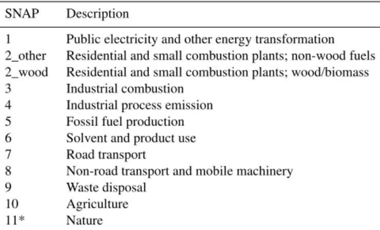
Ta-ble S1. The emission inventory database provides the emis-sions at a detailed level of about 200 sub-source categories. Each subcategory was spatially distributed using the most appropriate proxy map and then aggregated to Standardized Nomenclature for Air Pollutants (SNAP) level 1 source cate-gories (Table 1).
2.1.1 Primary PM10, PM2.5and PM1emission
inventory and EC and OC fractions
Size-fractionated EC and OC emission factors (carbonaceous mass per unit of activity) are available only for a limited number of sources and technologies and can vary widely due to different measurement protocols and analytical tech-niques (Watson et al., 2005). Although a direct calcula-tion of emissions as activity times the EC/OC emission fac-tor would be preferable, this would give widely varying, inconsistent and incomplete results. This problem is tack-led by starting from a size-fractionated particulate matter (PM10/PM2.5/PM1) emission inventory, followed by
deriv-ing and applyderiv-ing representative size-differentiated EC and OC fractions to obtain the EC and OC emissions in the size classes,<1, 1–2.5, and 2.5–10 µm.
A consistent set of PM10, PM2.5and PM1emission data
for Europe was obtained from the GAINS (Greenhouse Gas– Air Pollution Interactions and Synergies) model (Klimont et al., 2002; Kupiainen and Klimont, 2004, 2007). GAINS ac-counts for the effects of technology (such as emission con-trol measures) on PM emissions, which would otherwise be difficult to assess from the EC/OC literature. The detailed source categorization in GAINS enables the use of highly specific EC and OC fractions which increases the accuracy of the final emission inventory. For a description of the relevant GAINS PM emission data used here, we refer to Klimont et al. (2002) and Kupiainen and Klimont (2004, 2007). Fur-ther documentation can be found at the IIASA web page (http://www.iiasa.ac.at/). PM1, PM2.5 and PM10 emissions
by source sector often vary by country in GAINS, due to different degrees of emission control. The size-differentiated PM emission estimates (PM10, PM2.5, PM1) from GAINS
have been combined with EC and OC fractions, resulting in EC and OC emission estimates for 230 source categories and the three particle size classes.
Although EC and OC fractions may also vary with con-trol technology, the reviewed EC and OC literature does not allow further technology-dependent fractions of EC and OC. Therefore, EC and OC fractions were assumed to be indepen-dent of control technology. Since the absolute PM1, PM2.5
and PM10 emission level is control technology dependent,
Figure 1. PM2.5 EC and OC emissions (tonnes) for
UNECE-Europe in 2005 for each source sector (see Table 1) (excluding in-ternational shipping) according to the EUCAARI inventory and the TNO-newRWC.
et al. (2009) concentrated on adding new information if avail-able, and estimating the EC and OC fractions when no infor-mation was available.
The term EC is often used for measurements based on ther-mal analysis to indicate the carbon that does not oxidize be-low a certain temperature. OC refers to the non-carbonate carbonaceous material other than EC. OC content is usually expressed on a carbon mass basis. Full molecular mass (OM, organic matter) can be estimated by multiplication with a fac-tor to account for the other, non-C elements present in or-ganic matter like O and N; however, the OM/OC ratio varies
(Simon et al., 2011); freshly emitted primary organic aerosol typically have OM/OC ratios varying between about 1.2 and
1.8 (Aiken et al., 2008) and the ratio increases as the aerosol ages (OM/OC ratios of 2.5 have been observed for aged
am-bient oxygenated organic aerosol in Mexico; Aiken et al., 2008). Total carbon (TC) is the sum of EC and OC (C mass basis).
The IIASA GAINS PM emission data have been subject to a country consultation and review process and therefore for many countries these PM emissions are in line with na-tional reported emission data as available at the EMEP Cen-tre on Emission Inventories and Projections (CEIP) (http: //www.ceip.at/). The EUCAARI OA inventory (Fig. 1) was derived from the IIASA GAINS PM emission database in combination with the EC and OC fractions derived by Viss-chedijk et al. (2009).
2.2 Residential wood combustion in Europe
Wood, woody biomass and wood pellets are extensively used as fuel in European households. However, reliable fuel wood statistics are difficult to obtain because fuel wood is often non-commercial and falls outside the economic administra-tion. Therefore, fuel wood consumption has been notoriously underestimated in the past. Since combustion of wood is a key source of EC and OC we improved the available wood usage data through a stepwise approach. Specific wood use
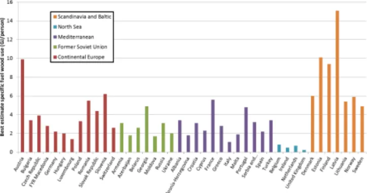
Figure 2.Estimated specific fuel wood use (in GJ person−1) in UNECE Europe grouped by region.
by country (GJ person−1)was primarily taken from GAINS. Estimates from the International Energy Agency (IEA, 2008) were used when GAINS data were lacking. By comparing in-dustrial and residential use of fuel wood in GAINS we con-clude that only the residential use is important on a Euro-pean scale; industry and power generation both consume less than 1 % of the total amount of wood used annually in Eu-rope (IEA, 2008; GAINS, 2009). Moreover, combustion ap-pliances in the residential sector have much higher PM emis-sion factors per unit of fuel. Therefore, our focus is on resi-dential combustion of wood and we neglect its minor use as a fuel in industrial combustion or power generation here.
Grouping the available statistical data resulted in five country cluster averages, based on geographical location and tradition, with wood use varying between 1.6 and 8.6 GJ person−1(Fig. 2). The observed differences between countries and country clusters can be related to the availabil-ity of local sources of fuel wood. We define “wood avail-ability” by the geographical intersection (arithmetic product) of population and local fuel wood sources, modelled by over-laying a map of gridded population on 1/16◦
Table 1.Description of source categories in the inventory.
SNAP Description
1 Public electricity and other energy transformation 2_other Residential and small combustion plants; non-wood fuels 2_wood Residential and small combustion plants; wood/biomass
3 Industrial combustion
4 Industrial process emission
5 Fossil fuel production
6 Solvent and product use
7 Road transport
8 Non-road transport and mobile machinery
9 Waste disposal
10 Agriculture
11* Nature
* Emissions for SNAP 11 (nature) are not included in the EUCAARI inventories. Modules for handling these biogenic are typically included in the chemical transport models.
The estimated residential fuel wood use by country is pre-sented in Fig. 2. Total wood use in UNECE Europe after reviewing the activity data and gap filling was about 20 % higher than the old data set.
Various types of appliances are used in Europe for resi-dential wood combustion and this has a significant impact on the EC/OC and PM emissions. In this study we adopt the split in appliance types given by Klimont et al. (2002) and Kupiainen and Klimont (2007) who distinguished seven ap-pliance types and provided relative shares of their use in dif-ferent countries. In terms of emission of particulate matter these technologies were ranked:
Fireplace > Conventional stove > Newer domestic
stoves and manual single house boilers>Automatic single
house boilers and 50–100 kW medium boilers>1–50 MW
Medium boilers.
Especially the fraction of fireplaces and conventional stoves has important implications for the PM/EC/OC emis-sion because of the corresponding relatively high emisemis-sion factors (Kupiainen and Klimont, 2007). For countries within our domain where no ratios between different appliances were given by Klimont et al. (2002) we used values for neigh-bouring or comparable countries (see Table S2). For several Eastern European countries the wood usage of fireplaces was reported as 0 %, we adjusted this by assuming 5 % applica-tion in fireplaces (the country cluster average). From the ac-tivity data for fuel wood consumption by appliance type by country, it is evident that Western European countries with a relatively high use of fuel wood also have the highest market penetration of more modern combustion equipment.
2.3 The TNO-newRWC emission inventory
The activity data described earlier, in combination with the adjusted allocation of wood by appliance type were used to develop a revised RWC emission inventory by selecting emission factors for each appliance type, independent of the country (Table 2). This is a first-order approach because it
neglects the importance of combustion conditions and “cul-tural” differences in how to burn wood. Nevertheless it leads to a more transparent and comparable emission inventory.
Emission factors for wood combustion vary widely even for the same appliance type. This is partly due to the influ-ence of combustion type, fuel parameters and different op-eration conditions. However, another important factor is the different sampling and measurement protocols or techniques. Nussbaumer et al. (2008a, b) made a detailed survey and re-view of the various emission factors in use in Europe, also in relation to the type of measurement technique. A total of 17 institutions from seven countries (Austria, Denmark, Ger-many, Norway, The Netherlands, Sweden and Switzerland) participated in the survey and contributed data to the ques-tionnaire. In addition, data for national emission factors were reported or gathered from the literature.
Nussbaumer et al. (2008a, b) describe various sampling methods and the respective emission factors. The most im-portant are filter measurements, measuring only solid parti-cles (SP), and dilution tunnel (DT) measurements, measuring solid particles and condensable organics (or semivolatile or-ganics). An example of the latter is the Norwegian standard NS 3058-2 which samples filterable particles in a dilution tunnel with a filter holder gas temperature at less than 35◦C and at small dilution ratios (DR) of the order 10. Due to the cooling, condensable organic material in the hot flue gas con-denses on the filter or the solid particles. The impact of the choice of SP or DT emission factors is large, as illustrated in detail in Table 2. For example, for conventional woodstoves, one of the most important categories in Europe, the average solid particle emission factor is 150 g GJ−1(range 49–650) whilst the average of the dilution tunnel measurements, that include both solid and condensable particles, is 800 g GJ−1 (range 290–1932). This implies a factor of 5 difference be-tween the absolute PM emissions depending on the choice to use an SP- or DT-based emission factor. National emission factors, used in official reporting, show a considerable range, even if they are of the same type (DT or SP), as is reflected in the range presented in Table 2 and documented in detail in Nussbaumer et al. (2008a, b). In the TNO-newRWC emis-sion inventory, the average DT emisemis-sion factors were used for the respective appliance types (Table 2); for all other EC and OC emissions sources the EUCAARI emission values (Visschedijk et al., 2009; Kulmala et al., 2011) remained un-changed; in Fig. 1 only the sector SNAP 2-wood is different. The result was a revised inventory with a consistent approach for residential wood combustion, independent of individual country emission factor choices used for official reporting. A detailed example is presented in Sect. 4.3.
It should be noted that we revised the primary PM10
Table 2.Wood use by appliance type in Europe in 2005 and related solid particle (SP) and dilution tunnel (DT) particle emission factors.
Appliance typea Wood use in Europe Fraction of wood Emission factor (g GJ−1)b
in 2005 (PJ) consumption SP DT
Avg Range Avg Range
Fire place 140 6 % 260 23–450 900 d
Traditional heating stove 1167 52 % 150 49–650 800 290–1932
Single house boiler automatic 198 9 % 30 11–60 60 d
Single house boiler manual 348 15 % 180 6–650 1000 100–2000
Medium boiler automatic 267 12 % 40 c 45 c
Medium boiler manual 141 6 % 70 30–350 80 30–350
Total Europe 2262 100 %
aFollowing IIASA GAINS stove type definition (Klimont, 2002). bDerived from Nussbaumer (2008a, b).
cRange in emission factor is determined by end-of-pipe emission control. dNot enough data available to indicate range.
These studies showed that the volatility distribution of the organic emissions can vary substantially, both between dif-ferent fuel and burner types and between difdif-ferent operation conditions/practices. To use a single volatility distribution for organic aerosol emissions for all types of residential biomass combustion as is done here, is a simplification.
2.3.1 Spatial distribution
To spatially distribute the emission from residential wood combustion we assumed that within a country the specific fuel wood use per inhabitant is higher in rural regions than in urban areas. The latter have more apartment and high-rise buildings, which often have no wood stoves and/or chimneys. This assumption is confirmed by overlaying gridded urban and rural population with the regional spatial distribution of wood combustion units for Sweden (D. Segersson, personal communication, 2008) and the Netherlands (ER, 2008). In both cases, the wood combustion unit distribution was based on chimney sweep statistics. For the Netherlands, a survey among clients of the wood stove sellers’ organization was also used. Overall, an urban house is about half as likely to be fitted with a wood combustion unit as a house in a rural environment. A factor of 2 difference may seem rather low, but this is an average value and it is consistent with data for Germany (Mantau and Sörgel, 2006).
Spatial distribution of wood use will also be influenced by the earlier discussed local wood availability that we derived by spatial analysis of population and woodland distribution. A relationship was derived between the country-specific fuel wood use (GAINS/IEA, see Sect. 2.2) and the summed wood availabilities of that country, as discussed in detail in Viss-chedijk et al. (2009). Thus the population contained in each cell of the population distribution grid was given a weight factor based on the surrounding woodland coverage. Taking local wood availability into account, and differentiating
be-tween urban and rural environments, leads to a distribution pattern that significantly deviates from the distribution of to-tal population. Further improvements in the distribution may be feasible by accounting for local factors such as legal re-strictions, cultural traditions and the connection of remote areas to energy distribution networks, but this has not been attempted within the present study.
3 Chemical transport modelling
Two chemical transport models are used in this study, the EMEP MSC-W and the PMCAMx models, both described below. As well as lending more robustness to this study (es-pecially for the modelling of such uncertain components as organic aerosol), these two models have different and com-plementary strengths. The EMEP model has been evaluated extensively in Europe for many pollutants and across many years (Jonson et al., 2006; Fagerli and Aas, 2008; Aas et al., 2012; Bergström et al., 2012; Genberg et al., 2013). The model is known to work well for compounds where the emis-sions are well characterized. The EMEP model is readily run for periods of many years, and in this study we will present results from annual simulations. PMCAMx has been widely evaluated in North America, but it has recently been shown to perform well also in Europe (Fountoukis et al., 2011). The model is typically run for shorter periods than EMEP (e.g. 1 month), and was evaluated against high time resolu-tion (1 h) measurements. PMCAMx has an advanced aerosol scheme, with full aerosol dynamics and a 10-bin sectional approach.
3.1 The EMEP MSC-W model
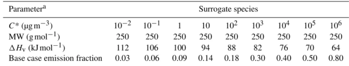
Table 3.Parameters used to simulate partitioning of primary organic aerosol in PMCAMx and EMEP MSC-W.
Parametera Surrogate species
C* (µg m−3) 10−2 10−1 1 10 102 103 104 105 106
MW (g mol−1) 250 250 250 250 250 250 250 250 250
1Hv(kJ mol−1) 112 106 100 94 88 82 76 70 64
Base case emission fraction 0.03 0.06 0.09 0.14 0.18 0.30 0.40 0.50 0.80
aC*: Saturation concentration at 298 K; MW: Molecular weight;1Hv: Enthalpy of vaporization.
aerosol chemistry (Simpson et al., 2012; Bergström et al., 2012). The model domain used in this study covers the whole of Europe, and includes a large part of the North Atlantic and Arctic areas, with a horizontal resolution of 50 km×50 km (at latitude 60◦N). The model includes 20 vertical lay-ers, using terrain-following coordinates; the lowest layer is about 90 m thick. Meteorological fields are derived from the ECMWF-IFS model (European Centre for Medium Range Weather Forecasting Integrated Forecasting System, http: //www.ecmwf.int/en/research/modelling-and-prediction).
The most recent version of the EMEP MSC-W model includes an organic aerosol scheme that uses the volatility basis set (VBS) approach (Donahue et al., 2009; Robinson et al., 2007) described in Sect. 3.3. An extensive sensitiv-ity analysis of this model has been presented by Bergström et al. (2012). In the present study we used an OA scheme with a nine-bin VBS for the primary OA (POA), including semivolatile and intermediate volatility (IVOC) gases (see Sect. 3.3 and Table 3). The IVOCs are missing in traditional OA and VOC emission inventories and for the standard emis-sion scenario (referred to as EUCAARI) the total emisemis-sions of semivolatile POA and IVOCs were assumed to amount to 2.5 times the POA inventory (based on Shrivastava et al., 2008) – that is, an IVOC mass of 1.5 times the POA emis-sions was added to the total emission input in the model. For the EMEP model simulations that used the revised RWC emissions, with emission factors based on dilution tunnel measurements, a slightly different emission split was applied for the RWC POA. We assumed that the DT methodology captures a larger fraction of the total semivolatile POA and IVOC emissions than traditional inventories (48 % for the new DT emissions, compared to 40 % for the EUCAARI emissions); the same volatility distribution of the OA sion was used in both cases but for the revised RWC emis-sion inventory total emisemis-sions are assumed to be 2.1 times the inventory (compared to the factor 2.5 for EUCAARI emis-sions).
The EMEP inputs used in the present study are based on Bergström et al. (2012) with a few updates. The most impor-tant changes are the following:
– The background concentration of organic aerosol is set to 0.4 µg m−3. Bergström et al. (2012) used a higher OA background concentration (1 µg m−3) but found that this
led to overestimations of OA at many sites during some periods.
– Emissions from open biomass fires (including vegeta-tion fires and open agricultural burning) are taken from the “Fire INventory from NCAR version 1.0” (FINNv1, Wiedinmyer et al., 2011).
– Hourly variations of anthropogenic emissions are used (as in Simpson et al., 2012); Bergström et al. (2012) used simple day–night factors.
The organic aerosol emissions from RWC (given as OC-emissions, in carbon units, in the inventories) are assumed to have an initial OM/OC ratio of 1.7 (based on data from
Aiken et al., 2008). Further details about the EMEP OA model setup are given by Bergström et al. (2012).
3.2 The PMCAMx model
of each species partitioned between the gas and aerosol phase is determined by applying the multicomponent aerosol ther-modynamic equilibrium model ISORROPIA-II (Fountoukis and Nenes, 2007) and is then distributed over the aerosol size sections by using weighting factors for each size section based on their surface area (Pandis et al., 1993).
The PMCAMx modelling domain covers a 5400× 5832 km2region in Europe with 36×36 km grid resolution and 14 vertical layers covering approximately 7 km with a surface layer thickness of 55 m. PMCAMx was set to per-form simulations on a rotated polar stereographic map pro-jection. The necessary inputs to the model include horizontal wind components, vertical diffusivity, temperature, pressure, water vapour, clouds and rainfall all created with the mete-orological model WRF (Weather Research and Forecasting). The biogenic emissions were produced by MEGAN (Model of Emissions of Gases and Aerosols from Nature) (Guenther et al., 2006). A marine aerosol emission model (O’Dowd et al., 2008) was also used for the estimation of mass fluxes for both accumulation and coarse mode including an organic fine-mode aerosol fraction. The model was successfully eval-uated against hourly aerosol mass spectrometry (AMS) data from various stations in Fountoukis et al. (2011) during a photochemically intense period. The model was also used to assess the importance of horizontal grid resolution and the use of high-resolution emissions on the predicted fine PM in a European Megacity (Fountoukis et al., 2013).
3.3 The volatility basis set framework
Both the EMEP MSC-W and PMCAMx models employ the volatility basis set (VBS) framework (Donahue et al., 2009; Robinson et al., 2007), using methods similar to those of Lane et al. (2008) and Shrivastava et al. (2008). Secondary organic aerosol (SOA) production from VOCs (Lane et al., 2008) is simulated using four semivolatile surrogate SOA products for each VOC, with four volatility bins (effective saturation concentrationsC∗of 1, 10, 100 and 1000 µg m−3 at 298 K). The models treat all organic aerosol species in the gas phase (primary and secondary) as chemically reac-tive. Each reaction with OH radical is assumed to decrease the volatility of the vapour material by a factor of 10 with a small net increase in mass (7.5 %) to account for added oxy-gen (Robinson et al., 2007). The primary OA emissions in the models were distributed by volatility (Table 3) using the volatility distributions of Shrivastava et al. (2008). This dis-tribution was derived by fitting gas particle partitioning data for diesel exhaust and wood smoke (Lipsky and Robinson, 2006; Shrivastava et al., 2006).
Primary organic gases, formed due to evaporation of semivolatile POA in the atmosphere, are assumed to react with OH radicals reducing their volatility. Chemical aging through gas-phase oxidation of primary OA vapours is mod-elled using a rate constant ofk=4×10⁻¹¹cm3molec−1s−1 (Atkinson and Arey, 2003).
4 Results, evaluation and discussion
The result of the work presented here was a revised RWC emission inventory as well as the use of that emission inven-tory in two CTMs and subsequent comparison with observa-tional data. These results are described and discussed in the following sections.
4.1 Revised RWC emission data
We constructed a revised bottom-up RWC emission inven-tory for Europe that also accounted for condensable organic material. Since EC is present as solid particles the change between the EUCAARI and TNO-newRWC for EC is rather small in most countries (Fig. 1; for a detailed discussion of the EC emissions see Genberg et al., 2013). However, for OC the change is large as most OC emissions are condens-able PM (Fig. 1). The revised RWC inventory changed the total primary OC emissions from wood combustion signifi-cantly but not in the same way for all countries. This is illus-trated in a more detailed comparison for selected countries in Fig. 3. Note that in this figure the sum of all anthropogenic OC sources are shown but the difference between the two bars for each country is only due to the new assessment of the wood-burning OC emissions.
The spatial distribution, using the new distribution proxy described in Sect. 2.3.1, of the European anthropogenic OC emissions is presented in Fig. 4. Important population cen-tres in countries with high wood consumption can be eas-ily recognized such as Oslo, Paris and Moscow, despite the fact that rural homes were allocated a relatively higher wood use. However, a distinct rural pattern can also be seen with for example high emissions in the eastern part of France. To give a spatial impression of the changes in emissions upon using the TNO-newRWC inventory we calculated the ra-tio of the revised emissions over the EUCAARI emissions (Fig. 5). The TNO-newRWC emissions are higher than the EUCAARI emissions in all countries except Norway. This is discussed in detail in Sect. 4.3.
Figure 3. Total organic carbon emissions (t C yr−1) for selected countries according to the EUCAARI and the TNO-newRWC emis-sion inventories.
Figure 4.Spatial distribution of the OC emissions (tonnes C/grid
cell; each cell is 1/8◦×1/16◦long–lat, ca 7×7 km) due to residential wood combustion in 2005 based on the TNO-newRWC inventory.
for the appliance types (Table 2) and their associated wood use for each country but no information how these appli-ance types are distributed within the country. Hence, within a country the fraction of each appliance type per grid cell is constant. This may not be realistic as, for example, more affluent regions may have more modern wood stoves. How-ever, we are not aware of reliable and documented data on this subject.
4.2 Chemical transport modelling results
The two CTMs were run with the two different RWC emis-sion inventories. Figure 6 shows the modelled OA concen-trations over Europe with the EUCAARI emission inven-tory, and the relative change in OA when using the revised RWC inventory instead. For the EUCAARI late winter/early spring AMS campaign (25 February–23 March 2009)
PM-Figure 5.Ratio of the revised TNO-newRWC inventory relative to
the previous EUCAARI OC emission inventory.
CAMx predicts mean OA concentrations of 1–2 µg m−3 in most of Europe and above 2 µg m−3in western France, Por-tugal, a fairly large region in western Russia and parts of the Baltic countries, and around some cities (e.g. Oslo, Lyon and Barcelona). The peak concentration, above 6 µg m−3, is predicted in the Paris area. The EMEP MSC-W model pre-dicts higher OA concentrations than PMCAMx in most of the modelling domain, above 2 µg m−3in most of southern and eastern Europe, and a remarkably high concentration in the Oslo region in southern Norway (above 4 µg m−3; a considerably higher level than anywhere in the neighbouring Nordic countries). However, in Paris and western France, the British Isles, Moscow, and the northernmost part of the do-main, EMEP gives lower concentrations than PMCAMx.
Both models show a significant increase in OA in large parts of Europe with the revised RWC inventory (and a substantial decrease in southern Norway). The response to changing the RWC emissions is larger in the EMEP model than in PMCAMx. For the February–March period, the EMEP model predicts more than 50 % higher total OA con-centrations with the revised RWC inventory than the old one in large parts of central and southern Europe, and Latvia, Lithuania and southern Finland. The impacts of changing the RWC emissions are much more “local” (and, especially for southern Europe, smaller) for PMCAMx than for EMEP (at least for the areas with increasing emissions); this indicates that the wood burning OA is removed more rapidly in PM-CAMx than in the EMEP MSC-W model.
−10 0 10 20 30 40 35 40 45 50 55 60 65 70 1.0 1.5 2.0 3.0 4.0 6.0 10.0 15.0
(a)OA, PMCAMx-Feb-Mar
−10 0 10 20 30 40 35 40 45 50 55 60 65 70 1.0 1.5 2.0 3.0 4.0 6.0 10.0 15.0
(b)OA, EMEP-Feb-Mar
−10 0 10 20 30 40 35 40 45 50 55 60 65 70 1.0 1.5 2.0 3.0 4.0 6.0 10.0 15.0
(c)OA, EMEP-Ann.
−10 0 10 20 30 40 35 40 45 50 55 60 65 70 1.0 1.5 2.0 3.0 4.0 6.0 10.0 15.0
−10 0 10 20 30 40 35 40 45 50 55 60 65 70 0.5 0.7 0.9 1.0 1.1 1.3 1.5 2.0 2.5
(d)Ratio, PMCAMx-Feb-Mar
−10 0 10 20 30 40 35 40 45 50 55 60 65 70 0.5 0.7 0.9 1.0 1.1 1.3 1.5 2.0 2.5
(e)Ratio, EMEP-Feb-Mar
−10 0 10 20 30 40 35 40 45 50 55 60 65 70 0.5 0.7 0.9 1.0 1.1 1.3 1.5 2.0 2.5
(f )Ratio, EMEP-Ann.
−10 0 10 20 30 40 35 40 45 50 55 60 65 70 0.5 0.7 0.9 1.0 1.1 1.3 1.5 2.0 2.5
Figure 6.Calculated near-surface organic aerosol (OA, top row) with the EUCAARI emission inventory (unit: µg m−3), for(a)PMCAMx model, February–March,(b)EMEP MSC-W February–March and(c)EMEP MSC-W annual, along with the ratio of calculated OA
(bottom-row) from TNO-new-RWC/EUCAARI, for(d)PMCAMx, February–March,(e)EMEP February–March,(f)EMEP annual. The February–
March period is 25 February–23 March 2009, the annual period is 1 January–31 December 2009.
RWC has a strong seasonal variation with the largest emis-sions during the cold seasons. In the EMEP MSC-W model about 80 % of the RWC emissions occur during the winter half-year, November–April. During the warmer months other sources of OC are more important (especially secondary or-ganic aerosol from oxidized biogenic VOC). It is difficult to model the boundary layer height accurately in large-scale CTMs and there is a risk that the models will underestimate PM from residential wood combustion (and other local, low stack-height sources) during calm, cold nights with strong temperature inversions. However, using the EMEP MSC-W model we find essentially no correlation between either mix-ing height or temperature and model bias for OC (see Sup-plementary information).
The modelled OC is in better agreement with observa-tions at most sites when using the revised RWC emissions compared to the EUCAARI emissions (Fig. 7, Table 4 and Supplement Fig. S1). The model–measurement correlation is higher with the revised inventory, at all of the five inves-tigated sites in the countries with large increases in RWC emissions (the average correlation coefficient,r, for the
win-ter half-year data, is 0.69 with the EUCAARI inventory and 0.75 with the revised RWC inventory); the mean absolute er-ror (MAE) of the model OC is lower with the revised inven-tory, except in Hyytiälä, where it is slightly higher (the aver-age relative MAE for the five sites, for November–April data,
decreases from 52 to 42 % when updating the RWC emission inventory).
The Norwegian site Birkenes was also included in the comparison (Fig. S1); Birkenes is situated in the southern-most part of Norway and it is to a large extent influenced by range transport from other parts of Europe. The long-term average (cold-season) model results and statistics for this site are very similar with the old and revised RWC emis-sion inventories; the reduced Norwegian emisemis-sions are bal-anced by increased emissions in the neighbouring countries. The revised emission inventory leads to higher correla-tion between modelled and measured total OC concentra-tions and lower model MAE also when comparing to full-year data (Supplement Table S3). Since the measurements of OC are not source-specific, improved model predictions can be caused by the increased RWC-emissions compensat-ing for other misscompensat-ing OC emissions in the model. However, the fact that both winter and full-year results are improved, in combination with the strong seasonal variation of the RWC emissions, is an indication that the revised emissions are in-deed more realistic than the old ones.
Figure 8 shows a comparison of predicted (PMCAMx) vs. Observed (AMS) PM1 OA concentrations (Crippa et
Figure 7.Measured and modelled organic carbon concentrations (2007–2009, winter half-year data: November–April) at four sites: Hyytiälä
Figure 8.Comparison of predicted (PMCAMx) vs. observed (AMS) PM1OA (µg m−3) from seven measurement sites during the EUCAARI winter 2009 campaign (25 February–23 March). Each point is a daily average value. The dashed lines represent 2 : 1 and 1 : 2 lines.
Table 4.Evaluation of EMEP MSC-W model prediction results (with two different inventories for residential wood combustion emissions)
to data from observations during the winter half-years (November–April) in 2007–2009. Observed: average measured OC concentration; Model: average modelled OC concentration (for the periods with measurements, see footnotes); R2: coefficient of determination; MAE:
mean of absolute error. Units for Observed, Model and MAE: µg(C)m−3. The relative MAE=MAE/Observed is given in parentheses (in %).
EUCAARI emissions TNO new RWC emissions
Site Observed Model R2 MAE Model R2 MAE
Hyytiälä (FI)a 1.12 0.80 0.55 0.43 (38 %) 1.21 0.61 0.47 (42 %)
Aspvreten (SE)b 1.77 0.92 0.47 0.91 (51 %) 1.35 0.48 0.75 (43 %)
Vavihill (SE)c 1.68 0.92 0.28 0.84 (50 %) 1.30 0.43 0.56 (33 %)
Melpitz (DE)d 2.12 0.97 0.48 1.20 (57 %) 1.51 0.52 0.88 (41 %)
Overtoom (NL)e 2.37 0.91 0.62 1.52 (64 %) 1.34 0.76 1.16 (49 %)
Birkenes (NO)f 0.58 0.65 0.66 0.24 (41 %) 0.66 0.69 0.25 (42 %)
a14 February 2007–18 February 2008, 129 measurements: Measured OC
1, Model OC2.5, Aurela et al. (2011).
b18 April 2008–30 December 2009, 114 measurements: OC 10. c24 April 2008–31 December 2009, 29 measurements: OC
10, Genberg et al. (2011). d1 January 2007–31 December 2009, 544 measurements: OC
2.5.
eNote: Urban background station in Amsterdam (the station is not heavily influenced by RWC, and OC concentrations are similar to surrounding rural background sites, Schaap and Denier van der Gon, 2007), 18 February 2007–31 December 2008, 63 measurements: OC2.5.
f2 January 2007–29 December 2009, 140 measurements: OC 2.5.
emission inventory improves the model performance against the AMS data. The slope of the linear fit increases from 0.51 to 0.82 with the use of the revised inventory for RWC emis-sions. The average fractional bias is substantially reduced (from−0.3 to 0.1) with the use of the revised RWC
inven-tory. The model predicts 35 to 85 % higher OA concentra-tions as a result of the update in the RWC emission inventory.
4.3 A case study: Norway and Sweden
In order to test the revised RWC emission inventory in more detail we performed a case study using data from published source apportionment studies for the two neighbouring coun-tries Norway and Sweden. Genberg et al. (2011) measured levoglucosan (LG) levels at Vavihill, in southern Sweden,
Figure 9. Comparison of EMEP MSC-W model-predicted OC
(µg(C) m−3) from biomass burning (bbOC) (including OC from both residential wood combustion and open vegetation fires) to bbOC estimated from levoglucosan concentrations at Vavi-hill (southern Sweden). Blue bars: model calculated bbOC with the EUCAARI emission inventory; black: model bbOC with the revised TNO-newRWC emission inventory. Red bars show the measurement-estimated bbOC range (lower limit: 5.5×the mea-sured levoglucosan concentration, upper limit: 14×levoglucosan; the estimated range for the bbOC/levoglucosan ratio, 5.5–14, is taken from Szidat et al., 2009).
OC is also improved compared to measurements (Table 4 and Fig. S1).
We also compared predicted OC from wood burning to source apportionment data from winter campaigns in and near Gothenburg in Sweden (Szidat et al., 2009) and in the Oslo region in Norway (Yttri et al., 2011). A more exten-sive comparison to these campaigns (including other sources and both summer and winter periods) was done by Bergström et al. (2012); in the present study we focused on the wood-burning part and the impact of the choice of RWC emission inventory. The results are shown in Fig. 10. For the Norwe-gian sites (Oslo and Hurdal, 70 km NE of Oslo) modelling with the EUCAARI emission inventory led to large overesti-mations of wood-burning OC; results were clearly improved for both sites when the TNO-newRWC inventory was used. Model results for the Swedish campaign were quite different, with underestimated wood-burning OC with the EUCAARI inventory while the results with the revised RWC inventory were within the 10–90 percentile of the source apportionment estimate, based on the measurements, for the rural back-ground site Råö, but still somewhat underestimated for the urban background site (Gothenburg). The revised RWC in-ventory also improves model results for wood-burning EC at these sites as shown by Genberg et al. (2013).
Although the two source apportionment campaigns were relatively short, and limited to two regions, the model im-provement using the revised RWC emission inventory is con-sistent with the findings for modelling total OC over longer time periods. These results further support the need to update
Figure 10.Comparison of model calculated OC (µg(C) m−3) from wood burning (residential combustion+open vegetation fires) to source-apportionment data from measurement campaigns during winter in Norway (SORGA, 1–8 March 2007, Yttri et al., 2011) and Sweden (GÖTE, 11 February–4 March 2005, Szidat et al., 2009).
and harmonize the official estimates of wood-burning emis-sions in Europe.
5 Conclusions and discussion
Combustion of biofuels, like wood, for cooking or heating is one of the major global sources of organic aerosol (OA). In Europe, residential wood combustion (RWC) is the largest source of OA. Robinson et al. (2007) proposed an alterna-tive framework for the treatment of OA in regional chemistry transport models (CTMs), commonly known as the Volatil-ity Basis Set approach. This acknowledged the semivolatile nature of OA and significantly improved our ability to re-produce observed OA concentrations. However, these new insights have so far had no, or little, impact on the primary particulate matter emission inventories used in Europe. In our opinion this issue needs to be addressed. Currently RWC is increasing in Europe because of rising fossil fuel prices and stimulation of renewable fuels in the framework of climate change mitigation policies. On the basis of the work pre-sented here we conclude that European emissions from RWC are significantly underestimated.
dilution of the flue gas or exhaust. We note that Murphy et al. (2014) suggest that in a simplified framework all emit-ted semivolatile organics (effective saturation concentration,
C∗, in the range 0.32–320 µg m−3) should be considered as primary OA.
In this study we adjusted only the RWC emissions while keeping other sources constant. The total European OA emis-sion estimates increased by almost a factor of 2. This will have important implications for PM2.5emissions as OA is an
important contributor to PM. Interestingly, the EEA/EMEP emission inventory guidebook (EEA, 2013b) was recently updated for wood combustion PM emission factors. We anal-ysed the new emission factors and conclude that they are in line with what was used in this study. For example, for the most important appliance type, the conventional wood stove (about 50 % of all wood consumption), the emission factor (DT) used in the TNO-newRWC is 800 g(PM)GJ−1 wood. EEA/EMEP (EEA, 2013b) presents exactly the same value but as total suspended particles (TSP) with the remark that PM2.5≈90–95 % of TSP. This is very similar compared
to the previous gap of a factor 2–4. There are also a few larger differences, e.g. our emission factor for conventional log boilers is a factor 2 higher than EEA/EMEP. However, given the ranges in emission factors shown in Table 2 this is not surprising. A quick calculation suggested that the TNO-newRWC emissions for RWC are likely to be only slightly higher (∼10–15 %) than when all countries would apply the new EEA/EMEP guidebook factors. As we have shown, this leads to a factor 2–3 higher emissions from RWC than cur-rently reported. It will increase total European PM2.5
emis-sions by about 20 %. Those are dramatic changes, and this will certainly help reducing the gap between modelled and observed PM, which has often been reported during cold sea-sons (Aas et al., 2012).
The Supplement related to this article is available online at doi:10.5194/acp-15-6503-2015-supplement.
Acknowledgements. Most measured campaign data originate from
EUCAARI partners (Kulmala et al., 2011). Most of the long-term OC filter measurement data were downloaded from the EBAS database (http://ebas.nilu.no); thanks to Hans Areskoug for OC data from Aspvreten, Dave de Jonge for OC data from Overtoom, Gerald Spindler for OC data from Melpitz, Karl Espen Yttri for OC data from Birkenes and Johan Genberg for OC data from Vavihill. OC data from Hyytiälä were provided directly by Sanna Saarikoski, of the Finnish Meteorological Institute. This work has been partly funded by EUCAARI (European FP6 No. 036833-2) and by the Swedish Clean Air Research Program (SCARP). S. N. Pandis and C. Fountoukis acknowledge support by the European Community’s 7th Framework Programme EU project PEGASOS (contract 265307).
Edited by: S. Galmarini
References
Aas, W., Tsyro, S., Bieber, E., Bergström, R., Ceburnis, D., Eller-mann, T., Fagerli, H., Frölich, M., Gehrig, R., Makkonen, U., Nemitz, E., Otjes, R., Perez, N., Perrino, C., Prévôt, A. S. H., Putaud, J.-P., Simpson, D., Spindler, G., Vana, M., and Yttri, K. E.: Lessons learnt from the first EMEP intensive measurement periods, Atmos. Chem. Phys., 12, 8073–8094, doi:10.5194/acp-12-8073-2012, 2012.
Aiken, A. C., Decarlo, P. F., Kroll, J. H., Worsnop, D. R., Huff-man, J. A., Docherty, K. S., Ulbrich, I. M., Mohr, C., Kimmel, J. R., Sueper, D., Sun, Y., Zhang, Q., Trimborn, A., Northway, M., Ziemann, P. J., Canagaratna, M. R., Onasch, T. B., Alfarra, M. R., Prevot, A. S. H., Dommen, J., Duplissy, J., Metzger, A., Baltensperger, U., and Jimenez, J. L.: O/C and OM/OC ratios of
primary, secondary, and ambient organic aerosols with high res-olution time-of-flight aerosol mass spectrometry, Environ. Sci. Technol., 42, 4478–4485, doi:10.1021/es703009q, 2008. Atkinson, R. and Arey, J.: Atmospheric degradation of volatile
or-ganic compounds, Chem. Rev., 103, 4605–4638, 2003.
Aurela, M., Saarikoski, S., Timonen, H., Aalto, P., Keronen, P., Saarnio, K., Teinilä, K., Kulmala, M., and Hillamo, R.: Car-bonaceous aerosol at a forested and an urban background sites in Southern Finland, Atmos. Environ., 45, 1394–1401, 2011. Berge, E. and Jakobsen, H. A.: A regional scale multi-layer model
for the calculation of longterm transport and deposition of air pollution in Europe, Tellus, 50, 205–223, 1998.
Bergström, R., Denier van der Gon, H. A. C., Prévôt, A. S. H., Yttri, K. E., and Simpson, D.: Modelling of organic aerosols over Eu-rope (2002–2007) using a volatility basis set (VBS) framework: application of different assumptions regarding the formation of secondary organic aerosol, Atmos. Chem. Phys., 12, 8499–8527, doi:10.5194/acp-12-8499-2012, 2012.
Biswas, S., Verma, V., Schauer, J. J., Cassee, F. R., Cho, A. K., and Sioutas, C.: Oxidative potential of semi-volatile and non-volatile particulate matter (PM) from heavy-duty vehicles retrofitted with emission control technologies, Environ. Sci. Technol., 43, 3905– 3912, 2009.
Bond, T. C., Streets, D. G., Yarber, K. F., Nelson, S. M., Woo, J., and Klimont, Z.: A technology based global inventory of black and organic carbon emissions from combustion, J. Geophys.Res., 109, D14203, doi:10.1029/2003JD003697, 2004.
Bond, T. C., Doherty, S. J., Fahey, D. W., Forster, P. M., Berntsen, T., DeAngelo, B. J., Flanner, M. G., Ghan, S., Kärcher, B., Koch, D., Kinne, S., Kondo, Y., Quinn, P. K., Sarofim, M. C., Schultz, M. G., Schulz, M., Venkataraman, C., Zhang, H., Zhang, S., Bellouin, N., Guttikunda, S. K., Hopke, P. K., Jacobson, M. Z., Kaiser, J. W., Klimont, Z., Lohmann, U., Schwarz, J. P., Shindell, D., Storelvmo, T., Warren, S. G., and Zender, C. S.: Bounding the role of black carbon in the climate system: a sci-entific assessment, J. Geophys. Res.-Atmos., 118, 5380–5552, doi:10.1002/jgrd.50171, 2013.
Prévôt, A. S. H.: Organic aerosol components derived from 25 AMS data sets across Europe using a consistent ME-2 based source apportionment approach, Atmos. Chem. Phys., 14, 6159– 6176, doi:10.5194/acp-14-6159-2014, 2014.
Denier van der Gon, H. A. C., Visschedijk, A., Van der Brugh, H., and Dröge, R.: A high resolution European emission database for the year 2005, a contribution to the UBAproject PAREST: Particle Reduction Strategies, TNO report TNO-034-UT-2010-01895_RPTML, published by the German Federal Environment Agency (Umweltbundesamt) as Texte 41/2013, Utrecht, avail-able at: http://www.umweltbundesamt.de/en/publications (last access: June 2014), 2010.
Donahue, N. M., Robinson, A. L., and Pandis, S. N.: Atmospheric organic particulate matter: from smoke to secondary organic aerosol, Atmos. Environ., 43, 94–106, 2009.
Echalar, F., Artaxo, P., Martins, J. V., Yamasoe, M., Gerab, F., Maenhaut, W., and Holben, B.: Long-term monitoring of atmo-spheric aerosols in the Amazon Basin: Source identification and apportionment, J. Geophys. Res.-Atmos., 103, 31849–31864, 1998.
EEA (European Environment Agency): European Union emission inventory report 1990–2011 under the UNECE Convention on Long-range Transboundary Air Pollution (LRTAP), EEA Techni-cal report No. 10/2013, doi:10.2800/44480, Copenhagen, 2013a. EEA (European Environment Agency): EMEP/EEA air pollutant emission inventory guidebook 2013, EEA Technical report No. 12/2013, doi:10.2800/92722, Luxembourg, 2013b.
ENVIRON: User’s Guide to the Comprehensive Air Quality Model with Extensions (CAMx), Version 4.02, Report, ENVIRON Int. Corp., Novato, Calif, available at: http://www.camx.com (last ac-cess: September 2014), 2003.
ER (The Netherlands Pollutant Release & Transfer Register): Grid-ded emission from residential wood combustion in the Nether-lands 2008, The NetherNether-lands Pollutant Release & Transfer Reg-ister, available at: http://www.emissieregistratie.nl, last access: March 2008.
Fagerli, H. and Aas, W.: Trends of nitrogen in air and pre-cipitation: model results and observations at EMEP sites in Europe, 1980–2003, Environ. Pollut., 154, 448–461, doi:10.1016/j.envpol.2008.01.024, 2008.
Fahey, K. and Pandis, S. N.: Optimizing model performance: vari-able size resolution in cloud chemistry modeling, Atmos. Envi-ron., 35, 4471–4478, 2001.
Fountoukis, C. and Nenes, A.: ISORROPIA II: a computa-tionally efficient thermodynamic equilibrium model for K+– Ca2+–Mg2+–NH+
4–Na+–SO24−–NO−3–Cl−–H2O aerosols,
At-mos. Chem. Phys., 7, 4639–4659, doi:10.5194/acp-7-4639-2007, 2007.
Fountoukis, C., Racherla, P. N., Denier van der Gon, H. A. C., Polymeneas, P., Charalampidis, P. E., Pilinis, C., Wiedensohler, A., Dall’Osto, M., O’Dowd, C., and Pandis, S. N.: Evaluation of a three-dimensional chemical transport model (PMCAMx) in the European domain during the EUCAARI May 2008 cam-paign, Atmos. Chem. Phys., 11, 10331–10347, doi:10.5194/acp-11-10331-2011, 2011.
Fountoukis, C., Koraj, D., Denier van der Gon, H. A. C., Charalam-pidis, P. E., Pilinis, C., and Pandis, S. N.: Impact of grid resolu-tion on the predicted fine PM by a regional 3-D chemical trans-port model, Atmos. Environ., 68, 24–32, 2013.
GAINS: Greenhouse gas and Air pollution Interaction Model, IIASA, Laxenburg, available at: http://gains.iiasa.ac.at/models/ (last access: September 2014), 2009.
Gaydos, T., Koo, B., and Pandis, S. N.: Development and applica-tion of an efficient moving secapplica-tional approach for the soluapplica-tion of the atmospheric aerosol condensation/evaporation equations, Atmos. Environ., 37, 3303–3316, 2003.
Gelencsér, A., May, B., Simpson, D., Sánchez-Ochoa, A., Kasper-Giebl, A., Puxbaum, H., Caseiro, A., Pio, C., and Legrand, M.: Source apportionment of PM2.5 organic aerosol over Europe: primary/secondary, natural/anthropogenic, fossil/biogenic origin, J. Geophys. Res., 112, D23S04, doi:10.1029/2006JD008094, 2007.
Genberg, J., Hyder, M., Stenström, K., Bergström, R., Simpson, D., Fors, E. O., Jönsson, J. Å., and Swietlicki, E.: Source apportionment of carbonaceous aerosol in southern Sweden, Atmos. Chem. Phys., 11, 11387–11400, doi:10.5194/acp-11-11387-2011, 2011.
Genberg, J., Denier van der Gon, H. A. C., Simpson, D., Swi-etlicki, E., Areskoug, H., Beddows, D., Ceburnis, D., Fiebig, M., Hansson, H. C., Harrison, R. M., Jennings, S. G., Saarikoski, S., Spindler, G., Visschedijk, A. J. H., Wiedensohler, A., Yt-tri, K. E., and Bergström, R.: Light-absorbing carbon in Eu-rope – measurement and modelling, with a focus on residential wood combustion emissions, Atmos. Chem. Phys., 13, 8719– 8738, doi:10.5194/acp-13-8719-2013, 2013.
Grieshop, A. P., Logue, J. M., Donahue, N. M., and Robinson, A. L.: Laboratory investigation of photochemical oxidation of or-ganic aerosol from wood fires 1: measurement and simulation of organic aerosol evolution, Atmos. Chem. Phys., 9, 1263–1277, doi:10.5194/acp-9-1263-2009, 2009.
Guenther, A., Karl, T., Harley, P., Wiedinmyer, C., Palmer, P. I., and Geron, C.: Estimates of global terrestrial isoprene emissions using MEGAN (Model of Emissions of Gases and Aerosols from Nature), Atmos. Chem. Phys., 6, 3181–3210, doi:10.5194/acp-6-3181-2006, 2006.
Hansen, J. E. and Sato, M.: Trends of measured climate forcing agents, P. Natl. Acad. Sci. USA, 98, 14778–14783, 2001. Heringa, M. F., DeCarlo, P. F., Chirico, R., Tritscher, T., Dommen,
J., Weingartner, E., Richter, R., Wehrle, G., Prévôt, A. S. H., and Baltensperger, U.: Investigations of primary and secondary particulate matter of different wood combustion appliances with a high-resolution time-of-flight aerosol mass spectrometer, At-mos. Chem. Phys., 11, 5945–5957, doi:10.5194/acp-11-5945-2011, 2011.
Hitzenberger. R. and Tohno, S.: Comparison of black carbon (BC) aerosols in two urban areas – concentrations and size distribu-tions, Atmos. Environ., 35, 2153–2167, 2001.
Hoek, G., Brunekreef, B., Goldbohm, S., Fischer, P., and van den Brandt, P. A.: Association between mortality and indicators of traffic-related air pollution in the Netherlands: a cohort study, Lancet, 360, 1203–1209, 2002.
IEA, International Energy Agency: World Energy Statistics and Balances (2008 Edition), IEA, Paris, France, 2008.
Jacobson, M. Z.: Strong radiative heating due to the mixing state of black carbon in atmospheric aerosols, Nature, 409, 695–697, 2001.
H. R., Brunekreef, B., and Cassee, F. R.: Black carbon as an addi-tional indicator of the adverse health effects of airborne particles compared with PM10 and PM2.5, Environ. Health Persp., 119, 1691–1699, doi:10.1289/ehp.1003369, 2011.
Jimenez, J. L., Canagaratna, M. R., Donahue, N. M., Prévôt, A. S. H., Zhang, Q., Kroll, J. H., DeCarlo, P. F., Allan, J. D., Coe, H., Ng, N. L., Aiken, A. C., Docherty, K. S., Ulbrich, I. M., Grieshop, A. P., Robinson, A. L., Duplissy, J., Smith, J. D., Wilson, K. R., Lanz, V. A., Hueglin, C., Sun, Y. L., Tian, J., Laaksonen, A., Raatikainen, T., Rautiainen, J., Vaattovaara, P., Ehn, M., Kulmala, M., Tomlinson, J. M., Collins, D. R., Cubi-son, M. J., Dunlea, E. J., Huffman, J. A., Onasch, T. B., Al-farra, M. R., Williams, P. I., Bower, K., Kondo, Y., Schnei-der, J., Drewnick, F., Borrmann, S.,Weimer, S., Demerjian, K., Salcedo, D., Cottrell, L., Griffin, R., Takami, A., Miyoshi, T., Hatakeyama, S., Shimono, A., Sun, J. Y., Zhang, Y. M., Dzepina, K., Kimmel, J. R., Sueper, D., Jayne, J. T., Herndon, S. C., Trim-born, A. M., Williams, L. R., Wood, E. C., Middlebrook, A. M., Kolb, C. E., Baltensperger, U., and Worsnop, D. R.: Evolution of organic aerosols in the atmosphere, Science, 326, 1525–1529, doi:10.1126/science.1180353, 2009.
Jonson, J. E., Simpson, D., Fagerli, H., and Solberg, S.: Can we ex-plain the trends in European ozone levels?, Atmos. Chem. Phys., 6, 51–66, doi:10.5194/acp-6-51-2006, 2006.
Junker, C. and Liousse, C.: A global emission inventory of car-bonaceous aerosol from historic records of fossil fuel and biofuel consumption for the period 1860–1997, Atmos. Chem. Phys., 8, 1195–1207, doi:10.5194/acp-8-1195-2008, 2008.
Kanakidou, M., Seinfeld, J. H., Pandis, S. N., Barnes, I., Dentener, F. J., Facchini, M. C., Van Dingenen, R., Ervens, B., Nenes, A., Nielsen, C. J., Swietlicki, E., Putaud, J. P., Balkanski, Y., Fuzzi, S., Horth, J., Moortgat, G. K., Winterhalter, R., Myhre, C. E. L., Tsigaridis, K., Vignati, E., Stephanou, E. G., and Wilson, J.: Organic aerosol and global climate modelling: a review, At-mos. Chem. Phys., 5, 1053–1123, doi:10.5194/acp-5-1053-2005, 2005.
Kiehl, J. T. and Briegleb, B. P.: The relative roles of sulfate aerosols and greenhouse gases in climate forcing, Science, 260, 311–314, 1993.
Klimont, Z., Cofala, J., Bertok, I., Amann, M., Heyes, C., and Gyarfas, F.: Modelling Particulate Emissions in Europe: a Frame-work to Estimate Reduction Potential and Control Costs, Interim Report IR-02-076, IIASA, Laxenburg, Austria, 2002.
Koo, B., Pandis, S. N., and Ansari, A.: Integrated approaches to modeling the organic and inorganic atmospheric aerosol compo-nents, Atmos. Environ., 37, 4757–4768, 2003.
Kuenen, J. J. P., Denier van der Gon, H. A. C., Visschedijk, A., Van der Brugh, H., and Van Gijlswijk, R.: MACC European emission inventory for the years 2003–2007, TNO report TNO-060-UT-2011-00588, TNO, Utrecht, 2011.
Kulmala, M., Asmi, A., Lappalainen, H. K., Baltensperger, U., Brenguier, J.-L., Facchini, M. C., Hansson, H.-C., Hov, Ø., O’Dowd, C. D., Pöschl, U., Wiedensohler, A., Boers, R., Boucher, O., de Leeuw, G., Denier van der Gon, H. A. C., Fe-ichter, J., Krejci, R., Laj, P., Lihavainen, H., Lohmann, U., Mc-Figgans, G., Mentel, T., Pilinis, C., Riipinen, I., Schulz, M., Stohl, A., Swietlicki, E., Vignati, E., Alves, C., Amann, M., Ammann, M., Arabas, S., Artaxo, P., Baars, H., Beddows, D. C. S., Bergström, R., Beukes, J. P., Bilde, M., Burkhart, J. F.,
Canonaco, F., Clegg, S. L., Coe, H., Crumeyrolle, S., D’Anna, B., Decesari, S., Gilardoni, S., Fischer, M., Fjaeraa, A. M., Foun-toukis, C., George, C., Gomes, L., Halloran, P., Hamburger, T., Harrison, R. M., Herrmann, H., Hoffmann, T., Hoose, C., Hu, M., Hyvärinen, A., Hõrrak, U., Iinuma, Y., Iversen, T., Josipovic, M., Kanakidou, M., Kiendler-Scharr, A., Kirkevåg, A., Kiss, G., Klimont, Z., Kolmonen, P., Komppula, M., Kristjánsson, J.-E., Laakso, L., Laaksonen, A., Labonnote, L., Lanz, V. A., Lehtinen, K. E. J., Rizzo, L. V., Makkonen, R., Manninen, H. E., McMeek-ing, G., Merikanto, J., Minikin, A., Mirme, S., Morgan, W. T., Nemitz, E., O’Donnell, D., Panwar, T. S., Pawlowska, H., Pet-zold, A., Pienaar, J. J., Pio, C., Plass-Duelmer, C., Prévôt, A. S. H., Pryor, S., Reddington, C. L., Roberts, G., Rosenfeld, D., Schwarz, J., Seland, Ø., Sellegri, K., Shen, X. J., Shiraiwa, M., Siebert, H., Sierau, B., Simpson, D., Sun, J. Y., Topping, D., Tunved, P., Vaattovaara, P., Vakkari, V., Veefkind, J. P., Viss-chedijk, A., Vuollekoski, H., Vuolo, R., Wehner, B., Wildt, J., Woodward, S., Worsnop, D. R., van Zadelhoff, G.-J., Zardini, A. A., Zhang, K., van Zyl, P. G., Kerminen, V.-M., Carslaw, K., and Pandis, S. N.: General overview: European Integrated project on Aerosol Cloud Climate and Air Quality interactions (EUCAARI) – integrating aerosol research from nano to global scales, Atmos. Chem. Phys., 11, 13061–13143, doi:10.5194/acp-11-13061-2011, 2011.
Kupiainen, K. and Klimont, Z.: Primary Emissions of Submicron and Carbonaceous Particles in Europe and the Potential for their Control, IIASA IR 04-079, IIASA, Laxenburg, Austria, 2004. Kupiainen, K. and Klimont, Z.: Primary emissions of fine
car-bonaceous particles in Europe, Atmos. Environ., 41, 2156–2170, 2007.
Lane, T. E., Donahue, N. M., and Pandis, S. N.: Simulating sec-ondary organic aerosol formation using the volatility basis-set approach in a chemical transport model, Atmos. Environ., 42, 7439–7451, 2008.
Lipsky, E. M. and Robinson, A. L.: Effects of dilution on fine parti-cle mass and partitioning of semivolatile organics in diesel ex-haust and wood smoke, Environ. Sci. Technol., 40, 155–162, 2006.
Mantau, U. and Sörgel, C.: Energieholzverwendung in privaten Haushalten, Marktvolumen und verwendete Holzsortimente – Abschlußbericht, Zentrum Holzwirtschaft, Universität Hamburg, Hamburg, 2006.
Miller, K. A., Siscovick, D. S., Sheppard, L., Shepherd, K., Sul-livan, J. H., Anderson, G. L., and Kaufman, J. D.: Long-term exposure to air pollution and incidence of cardiovascular events in women, New Engl. J. Med., 356, 447–458, 2007.
Murphy, B. N., Donahue, N. M., Robinson, A. L., and Pandis, S. N.: A naming convention for atmospheric organic aerosol, At-mos. Chem. Phys., 14, 5825–5839, doi:10.5194/acp-14-5825-2014, 2014.
Myhre, G., Stordal, F., Restad, K., and Isaksen, I. S. A.: Estimation of the direct radiative forcing due to sulfate and soot aerosols, Tellus B, 50, 463–477, 1998.
Nussbaumer, T., Klippel, N., and Johansson, L.: Survey on Mea-surements and Emission Factors on Particulate Matter from Biomass Combustion in IEA Countries, 16th European Biomass Conference and Exhibition, Valencia, Spain, 2–6 June 2008, Oral Presentation OA 9.2, 2008b.
O’Dowd, C. D., Langmann, B., Varghese, S., Scannell, C., Ce-burnis, D., and Facchini, M. C.: A combined organic–inorganic sea-spray source function, Geophys. Res. Lett., 35, L01801, doi:10.1029/2007GL030331, 2008.
Pandis, S. N., Wexler, A. S., and Seinfeld, J. H.: Secondary organic aerosol formation and transport. 2. Predicting the ambient sec-ondary organic aerosol size distribution, Atmos. Environ., 27A, 2403–2416, 1993.
Pouliot, G., Pierce, T., Denier van der Gon, H., Schaap, M., Moran, M., and Nopmongcol, U.: Comparing emission inventories and model-ready emission datasets between Europe and North Amer-ica for the AQMEII project, Atmos. Environ., 53, 4–14, 2012. Robinson, A. L., Donahue, N. M., Shrivastava, M. K., Weitkamp,
E. A., Sage, A. M., Grieshop, A. P., Lane, T. E., Pierce, J. R., and Pandis, S. N.: Rethinking organic aerosols: semivolatile emis-sions and photochemical aging, Science, 315, 1259–1262, 2007. Schaap, M. and Denier van der Gon, H. A. C.: On the variability of black smoke and carbonaceous aerosols in the Netherlands, Atmos. Environ., 41, 5908–5920, 2007.
Schaap, M., Denier Van Der Gon, H. A. C., Dentener, F. J., Viss-chedijk, A. J. H., Van Loon, M., ten Brink, H. M., Putaud, J.-P., Guillaume, B., Liousse, C., and Builtjes, P. J. H.: Anthropogenic black carbon and fine aerosol distribution over Europe, J. Geo-phys. Res., 109, D18207, doi:10.1029/2003JD004330, 2004. Shrivastava, M. K., Lipsky, E. M., Stanier, C. O., and Robinson,
A. L.: Modeling semivolatile organic aerosol mass emissions from combustion systems, Environ. Sci. Technol., 40, 2671– 2677, doi:10.1021/es0522231, 2006.
Shrivastava, M. K., Lane, T. E., Donahue, N. M., Pandis, S. N., and Robinson, A. L.: Effects of gas particle partitioning and aging of primary emissions on urban and regional or-ganic aerosol concentrations, J. Geophys. Res., 113, D18301, doi:10.1029/2007JD009735, 2008.
Simon, H., Bhave, P. V., Swall, J. L., Frank, N. H., and Malm, W. C.: Determining the spatial and seasonal variability in OM/OC
ratios across the US using multiple regression, Atmos. Chem. Phys., 11, 2933–2949, doi:10.5194/acp-11-2933-2011, 2011. Simoneit, B. R. T., Schauer, J. J., Nolte, C. G., Oros, D. R., Elias, V.
O., Fraser, M. P., Rogge, W. F., and Cass, G. R.: Levoglucosan, a tracer for cellulose in biomass burning and atmospheric particles, Atmos. Environ., 33, 173–182, 1999.
Simpson, D., Yttri, K., Klimont, Z., Kupiainen, K., Caseiro, A., Gelencsér, A., Pio, C., and Legrand, M.: Modeling carbona-ceous aerosol over Europe. Analysis of the CARBOSOL and EMEP EC/OC campaigns, J. Geophys. Res., 112, D23S14, doi:10.1029/2006JD008158, 2007.
Simpson, D., Benedictow, A., Berge, H., Bergström, R., Emberson, L. D., Fagerli, H., Flechard, C. R., Hayman, G. D., Gauss, M., Jonson, J. E., Jenkin, M. E., Nyíri, A., Richter, C., Semeena, V. S., Tsyro, S., Tuovinen, J.-P., Valdebenito, Á., and Wind, P.: The EMEP MSC-W chemical transport model – technical descrip-tion, Atmos. Chem. Phys., 12, 7825–7865, doi:10.5194/acp-12-7825-2012, 2012.
Skyllakou, K., Murphy, B. N., Megaritis, A. G., Fountoukis, C., and Pandis, S. N.: Contributions of local and regional sources to fine PM in the megacity of Paris, Atmos. Chem. Phys., 14, 2343– 2352, doi:10.5194/acp-14-2343-2014, 2014.
Streets, D. G., Gupta, S., Waldhoff, S. T., Wang, M. Q., Bond, T. C., and Yiyun, B.: Black carbon emissions in China, Atmos. En-viron., 35, 4281–4296, 2001.
Szidat, S., Ruff, M., Perron, N., Wacker, L., Synal, H.-A., Hallquist, M., Shannigrahi, A. S., Yttri, K. E., Dye, C., and Simpson, D.: Fossil and non-fossil sources of organic carbon (OC) and ele-mental carbon (EC) in Göteborg, Sweden, Atmos. Chem. Phys., 9, 1521–1535, doi:10.5194/acp-9-1521-2009, 2009.
Visschedijk, A., Denier van der Gon, H., Droge, R., and van der Brugh, H.: A European High Resolution and Size-Differentiated Emission Inventory for Elemental and Organic Carbon for the Year 2005, TNO-034-UT-2009-00688_RPT-ML, TNO, Utrecht, 2009.
Watson, J. G., Chow, J. C., and Chen, L.-W. A.: Summary of or-ganic and elemental carbon/ black carbon analysis methods and intercomparisons, Aerosol Air Qual. Res., 5, 65–102, 2005. WHO – Europe: Particulate Matter Air Pollution: How it Harms
Health, Fact sheet EURO/04/05, World Health Organization – Europe, Berlin, Copenhagen, Rome, 2005.
Wiedinmyer, C., Akagi, S. K., Yokelson, R. J., Emmons, L. K., Al-Saadi, J. A., Orlando, J. J., and Soja, A. J.: The Fire INventory from NCAR (FINN): a high resolution global model to estimate the emissions from open burning, Geosci. Model Dev., 4, 625– 641, doi:10.5194/gmd-4-625-2011, 2011.
Yttri, K. E., Simpson, D., Stenström, K., Puxbaum, H., and Svendby, T.: Source apportionment of the carbonaceous aerosol in Norway – quantitative estimates based on14C, thermal-optical and organic tracer analysis, Atmos. Chem. Phys., 11, 9375–9394, doi:10.5194/acp-11-9375-2011, 2011.