”Do Shocks Permanently Change Output? Local
Persistency in Economic Time Series”
Luiz Renato Lima
1Zhijie Xiao
2Abstract
While it is recognized that output uctuations are highly persistent over certain range, less persistent results are also found around very long horizons (Conchrane, 1988), indicating the existence of local or tempo-rary persistency. In this paper, we study time series with local persis-tency. A test for stationarity against locally persistent alternative is pro-posed. Asymptotic distributions of the test statistic are provided under both the null and the alternative hypothesis of local persistency. Monte Carlo experiment is conducted to study the power and size of the test. An empirical application reveals that many US real economic variables may exhibit local persistency.
1
Introduction
Since the in uential article by Nelson and Plosser (1982), hundreds of economic time series have been examined by unit root tests and empirical evidence has accumulated that many economic and financial time series contain a unit root. However, as argued elsewhere (see for example Kwiatkowski et al., 1992), many standard testing proce-dures consider the null hypothesis of a unit root which ensures that the null hypothesis is accepted unless there is strong evidence against it. Indeed, different results have been obtained from other approaches.
While it is recognized that many economic time series are persistent, less persistent results are also found around very long horizons (see, e.g., Beaudry and Koop 1993 Hess and Iwata 1997 Koenker and Xiao 2002), indicating the existence of “local per-sistency” in economic time series. For example, output uctuations may be persistent over a long range of time, but not forever and will eventually disappear (Conchrane, 1988).
In recent ten years, a large amount of literature have emphasized that many eco-nomic time series are better characterized by a process with root near unity rather than an exact unit root. In effect, Chang and Lai (1998) claim that most of real exchange rates of the G-7 countries has root near unity. Lanne (2000) claims that the dynamic of interest rates are better characterized by a process with a root near unity rather than a process with an exact unit root. Dutkowsky and McCoskey (2001) show that near-unit roots are also present in the spread between Federal Funds rate and the discount rate during the post-1987 period and they use this fact to show that structural restrictions are compatible with stationary borrowing and a spread with root near unity.
The simplest local to unity model is a triangular array for a time series of the
form
(1)
with iid innovations While the autoregressive coefficient as
it is apparent that for any given sample size in (1), the model accommodates a
wider range of autoregressive coefficients as the localizing parameter varies, including
both stationary ( explosive ( ) and unit root ( ) possibilities. This
exibility has helped to make the model popular in studying economic time series for which roots near unity are considered highly plausible but roots at unity are considered too restrictive. However, in the traditional local to unit root model, shocks are still permanent and can not capture the feature of local persistency.
In this paper, we use a new time series model recently proposed by Phillips et al. (2001) to capture local persistence. This new formulation of local to unity model of-fers more exibility than the traditional model (1). The new model leads to a class of different limit processes beyond simple diffusions and also provides a more complete
interface between and models and between and asymptotics.
We call this model a block local to unity model. This model generates processes with roots near unity and includes local persistency as a general case. By proposing a statis-tical test that can be used to detect the presence of local persistency in economic time series, this paper aim to provide a first step of study on locally persistent processes.
This paper is organized as follows: Section 2 presents the stochastic block local to unit process, developed by Phillips et al (2001). The locally persistent process is com-pared with the fractionally integrated process, which is a related but different process. The behavior of the impulse response function is also investigated in section 2. In sec-tion 3, we introduce a test through which we test the null hypothesis of stasec-tionarity against local persistency of near unit root processes and derive its asymptotic
distrib-ution under the null and alternative hypothesis. Section 4 presents some results of the
Monte Carlo experiments. An empirical study on the presence of local persistency in some US time series is conducted in Section 5. Section 6 concludes.
weak convergence, convergence in probability and equality in distribution, respectively. Following the standard stochastic order of magnitude notation, we write
and to signify that the sequence of random variable is bounded and
converges to zero, respectively, as the sample size, goes to infinite.
2
A Model with Local Persistency
2.1
Locally Persistent Process Without Drift
The time series that we consider is the following process
, , (2)
where the coefficient “ in the autoregression is near unity and measures the
persis-tency in time series . We allow the errors to be a general covariance stationary time
series which satisfies an invariance principle.
It can be verified that by a re-parameterization ( ) we may re-write the above
time series in the format of a block local to unit root model which was first introduced by Phillips et al (2001). For more discussions on regularity assumptions and asymptotic properties of the above time series, see Phillips et al (2001).
The process provides a new form of persistent behavior when . The
above device provides a statistical model for what may be described as “locally per-sistent behavior” for macroeconomic time series. Many macroeconomic time series are now well known to display a form of persistence whereby economic shocks have long-run effects. However, it is possible that shocks may affect an economy for a long period of time but not forever. In other words, the effects of a shock may be highly persistent over a certain range (the range of persistent behavior), but then may begin to disappear outside this range. In the above model, the largest autoregressive root of time
series is close to unity and thus persistency can be found in . On the other hand,
the series evolves over time in such a way that there is persistency over a range of time
(of order compared to the full sample range ), but the effect of shocks will
eventurelly disappear over time horizon longer than order . The region of
persis-tent behavior may constitute a ‘little infinity’ relative to the full sample. Since there is
persistent memory within a time horizon of order but there is only short
mem-ory over longer periods, we call this type of memmem-ory “local persistence” or “temporal persistence”. For this reason, we call the above process a Locally Persistent process with persistent parameter .
We are especially interested in the case that In this case, the process
stationary or unit root process. It is a locally persistent process. In particular,
implying that the process will ultimately diverge at rate as
However, the model does include traditional stationary process and the unit-root type persistency as two special extreme cases. In particular,
When it reduces to the traditional near-integrated processes and has the
conventional unit-root type persistency. In particular, shocks has permanent effects,
with diverging at rate See, inter alia, Phillips (1988), for properties of this
kind of process
When the process becomes standard stationary process
Locally persistent processes are not covariance-stationary and, as we will see soon, they may be used to model the dynamics of economic time series that display persis-tence as well as transitory shocks.
2.2
Locally Persistent Process With A Deterministic Trend
The locally persistent process can be extended to include a deterministic time trend. Such an extension is important because many economic time series display tendency of
growth. We may consider a locally persistent process with trend component
, , (3)
where is a deterministic trend, the leading case being a linear time trend where
The stochastic part represented by Eq. (3) corresponds to (2), a locally persistent process without trend.
Note that the trend coefficients are unknown and thus, in practice, appropriate
de-trending is needed. We may estimate from the residuals of the following detrending
regression
(4)
where is the least squares estimator of . The detrended time series has
proper-ties similar to the process with no drift
2.3
Local Persistency versus Long Memory
A related but different model is the long-memory, or fractional integrated process with
order of integration equal to 3 that is, FI(d) with . Both the locally persistent
process that we consider in this paper and the conventional fractional integrated process
are between the conventional covariance stationary process and unit root process. How-ever, these two process have important differences. In particular, the fractionally inte-grated process (FI(d)) is more appropriate to capture long-range dependence, and our local persistence process (LP(d)) captures regional persistence. We illustrate below the differences in terms of impulse response functions
2.3.1 The Behavior of the Impulse Response Function
An impulse response function traces the effect of a shock in the innovation on current
and future values of the endogenous variable . If the process is stationary,
then its impulse response will converge to zero as the response horizon increases and
we say that the shocks are transitory. On the other hand, when the process has a unit
root the impulse response never converges to zero. Thus, when the process is a random walk we say that the shocks are permanent implying that an initial shock never dies out. As an illustration, consider the following models:
Model 1 and
Model 2 and
Model 3
In all these models we assume that is an i.i.d sequence of innovations.
In Model 1, is stationary when . If the response horizon equals one
can show that the period impulse response as .
Therefore, if is stationary the shocks will be totally absorbed as increases. Also
notice that, according to model 1, the total impact of a unit innovation,
Now we consider Model 1 where has a unit root, that is, . In this random walk
specification, it is well known that for any (If is not an i.i.d. sequence,
then the impulse response function may move up and down but with no convergence toward zero.) The shocks never vanish when there is a unit root and, more importantly,
the total impact goes to infinity, that is,
Model 2 represents a fractional white noise process. This process can be expressed as an infinite order moving average representation,
Therefore for So, the impact of the
we have so that the total impact of a unit innovation is infinite
which is similar to the result obtained in the unit root case.
Now, we analyze the behavior of the impulse response function locally persistent processes. Consider the standardized locally persistent process given in Model 3 with
. The period impulse response is given by and we
can see that if for any ( if or
). Thus, the impulse response does not go to zero in relatively shorter period, but
disappears in longer horizon. For any time period that is proportional to the sample
size . In this sense, we say that if the process is locally persistent, its
impulse response eventually converges to zero and, therefore, the shocks are globally
transitory. Moreover one can see that as and, therefore, the
impact of innovations dissipates faster when the process is locally persistent than when it is a fractional white noise. Moreover, the degree of persistency is determined by the parameter : the larger d, the more persistent are the shocks and, therefore, we can affirm that shocks take much more time to die out when the process is locally persistent than when it is stationary. In the degenerate case of model (2) where
, the period impulse response function In this
case, the autoregressive coefficient converges to one at rate which is the same rate by
which the exponent goes to infinity. Thus, the coefficient is close enough to unity
to avoid the impulse response function converging to zero, and therefore
as 4. This is because that a nearly integrated process have same unit-root type
of persistency, that is, the shocks are not transitory.
Overall, we may say that a locally persistent process and a fractionally integrated process are similar in the sense that they are sitting in between the stationary and unit root extremes and their impulse responses converge to zero. However, it is important to stress that the total impact of a innovation will never be less than infinite if the process is fractionally integrated and this represents an important difference between local persistence and long memory. In practice, it may be more appropriate to think at a mean-reverting economic variable as a process in which the total impact of a unit innovation is finite. For example, techonological innovations (shocks) might trigger a persistent economic growth, but it would be hard to believe that the total impact of such innovations on the GDP is going to persist forever. As another example, if one says that the real exchange rate (RER) is neither I(0) nor I(1), then the purchasing power parity (PPP) holds no matter whether RER is fractionally integrated or locally persistent. However, a complete parity reversion would not take place at a finite time
period if real exchange rate is fractionally integrated since its impulse response function is decaying hyperbolically. On the other hand, full PPP reversion would occur in a finite time horizon if real exchange rate is locally persistent.
We have seen so far that the persistency parameter is important to determine the
extension of region of persistency of a locally persistent process. Hence, it turns out to
be important to discuss estimation of as well as testing related hypothesis. In the next
two sections, we discuss estimation of and propose a test for the null that the process
is stationary against the alternative with local persistency.
3
Estimation of the Local-Persistence Parameter.
According to local persistence process, the extension of region of persistency is given
by the magnitude of the parameter The greater the value of the longer the
per-sistent range and the longer the perper-sistent effect will last. Therefore, it turns out to be
important to estimate the parameter in order to identify the degree of local persistence
of the stochastic process. In order to do so, without changing the level of persistency (magnitude of ), we need to standardize the localizing parameter. For convenience, we consider a standardized LP process, in which the localizing parameter, , equals
. Notice that and after taking the logarithm , one obtains
(5)
Following Phillips et al (2001), after standardization, we have that:
(6) i.e.
(7) where
Therefore, is made up of two components. The first one corresponds to the usual
least-square estimator of . The second one is a nonparametric correction that uses
the consistent estimator of the one sided long run covariance parameter, .5 The
non-parametric correction is needed whenever we have a non i.i.d. innovation sequence
, where is a consistent estimator of the variance of and
When the innovation sequence is independent and identically distributed, we have
The above result implies that
! (8)
Hence, one can propose the following consistent estimator for
(9)
4
Testing the Null Hypothesis of Stationarity against
Lo-cal
Persistency
In this section, using the proposed models (2) and (3), we construct a test for the null
hypothesis of covariance stationarity," , against the alternative of local
per-sistency, that is," . Notice that under the null, the order of magnitude
of the partial sum process should be proportional to (although may
have high variance, it is not large in order of magnitude and can be normalized). Under
mild conditions ( ! ) satisfies an invariance principle. On the
other hand, if the time series is locally persistent as described by (2), the cumulated sum
process diverges to more rapidly than rate . This observation suggests
that it is possible to design a test by looking at the order of magnitude of the partial sum process.
We consider the following quantity as a measurement of the magnitude of the cu-mulated sum
# $ %
Under" the above quantity converges weakly to & ! where& !
interval, with variance' long-run variance of lim E
Under the alternative hypothesis, is a locally persistent, it is easy to verify that the
corresponding statistic has much larger order of magnitude, diverging to as .
Notice that in practical analysis the limiting distribution depends on the long-run
variance parameter' which is unknown and thus the above quantity can not be used
di-rectly. However,' can be consistently estimated using nonparametric kernel
smooth-ing. We denote the estimator for' as' . We propose the following two statistic for
testing the null hypothesis of stationarity or trend stationarity against local persistent nonstationarity
( # $
)
%
(10)
( # $
)
%
(11)
where( is the test statistic evaluated at the observable time series, , and( is the
test statistic evaluated at the detrended time series
Theorem 1: (asymptotic behavior of the test statistic( under the null, ) Let
be a process without a time trend as defined in (2). Under" and the
assumption of Phillips et al. (2001),
( # $
)
%
(12)
! * ! !*
Table II reproduces the critical values for the test statistic(
Table I: Upper Tail Critical Values for(
Level of significance 0.1 0.05 0.01
Critical value 1.22 1.36 1.63
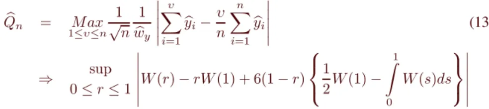
Theorem 2: (asymptotic behavior of the test statistic( under the null, ).
Let be a process with a time trend ( as defined in (3). Under" and
( # $ )
%
(13)
! * ! !* ! * * + +
where is the detrended value of
In Theorem 1, the test statistic converges to a functional of Brownian bridge.
The-orem 2, on the other hand, states that the test statistic( converges to the+ ,of the
Brownian bridge plus a second term brought of a time trend . Xiao (1999) calculated,
via simulation, the critical values for the test statistic( which is reproduced in the
table below.
Table II: Upper Tail Critical Values for(
Level of Significance 0.1 0.05 0.01
Critical value 0.827 0.901 1.041
It is critical that a statistical test be able to discriminate between the null and the alternative in large sample. The following Theorem gives properties of the tests under the alternative.
Theorem 3:(Consistency). Under the alternative hypothesis that" ,
,
,
Assuming that the bandwidth parameter- , then( and(
indicating that under the alternative hypothesis, the test statistic will reject the null with probability one.
Theorem 3 shows that if we choose- say,- the statistical test
proposed in this section is consistent since( and( diverge under the alternative
hypothesis as
4.1
Monte-Carlo Results
statistic( under" and" 6. From the construction of( we know that such
sta-tistics depends on the sample size , the parameter of persistency and the bandwidth
parameter-that is used to calculate) Consequently, we paid special attention to the
effects of and, - on the performance of this test. We considered the following
sample sizes: and These sample sizes represent the most
rel-evant range of sample sizes in many empirical analyses. Four bandwidth choices were
considered, the first two bandwidth values are small and fixed,- - while
the third bandwidth value- is function of the sample size and are increasing
with We used four values for the persistency parameter: The
first one corresponds to a process with local persistence but still close to stationarity, the second and third values represent processes with local persistence. The degenerate case, represents near integration and this process is supposed to diverge to infinity at
the same rate as a process with unit root, i.e., . All experiments used 10,000
replications. For the Kernel function, following Kwiatkowski et al. (1992), we used the
Bartlett window $ $ so that the nonnegativity of) was guaranteed.
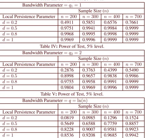
4.1.1 Power of Test
The data were generated from , where is a linear trend
with In each replication, we used the detrended value
of to calculate the value of the test statistic( 7 Theorem 3 predicts that we will
reject the null hypothesis with probability one when the sample size goes to infinity and" is true. For the four values of the local-persistence parameter the tables
below confirm what the theory predicts, that is, for any the probability
of rejecting" increases toward unity as the sample size increases. In particular, the
test exhibits low power when the process is near stationary, that is, when and the
sample size are small and , for example. . However, the power
of the test increases significantly whenever the presence of local persistence becomes more evident (i.e., when d increases). One can also see that the power is reduced as
the bandwidth parameter- increases because, as showed by theorem 3, the power of
our test depends upon - In other words, a large-will reduce the power, whereas a
large and a large will increase the power. All this is confirmed by the Monte-Carlo
results presented below.
We choose because the specification with linear trend represents the leading case in many applied works.
We also considered cases where displays serial correlation. In this case we modelled
where and The conclusion on power and
Table III:Power of Test, 5% level.
Bandwidth Parameter
-Sample Size ( ) Local Persistence Parameter
0.4911 0.5851 0.6576 0.7661
0.9751 0.9941 0.9984 0.9999
0.9968 0.9995 0.9998 0.9999
0.9969 0.9996 0.9999 0.9999
Table IV:Power of Test, 5% level.
Bandwidth Parameter
-Sample Size ( ) Local Persistence Parameter
0.2876 0.3763 0.4399 0.5490
0.8998 0.9657 0.9838 0.9986
0.9755 0.9958 0.9991 0.9999
0.9804 0.9969 0.9996 0.9999
Table V:Power of Test, 5% level.
Bandwidth Parameter
-Sample Size ( ) Local Persistence Parameter
0.0819 0.0985 0.1296 0.1524
0.5649 0.6588 0.7759 0.8857
0.8228 0.9007 0.9581 0.9923
0.8536 0.9208 0.9685 0.9942
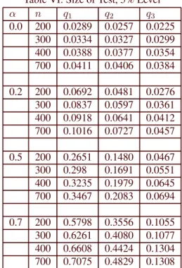
4.1.2 Size of Test
We next examined the size properties of( under the null hypothesis. For this purpose,
the data were generated from , where is a linear trend
with In this model, is not assumed to be local to unity and,
there-fore, it will not converge to unity as the sample size increases. Thus, if we choose an
appropriate bandwidth parameter-, we could expect that the size of test would converge
to the nominal size as the sample size increases. Notice, however, that the bandwidth
parameter-corresponds to the number of lags used to calculate ) . Intuitively, for
, the larger is, the longer lags we need. In the case that is an
inde-pendent sequence and the long-run variance of equals the variance of Thus, we
expect that for small a small bandwidth parameter would be more appropriate than a
for the existence of serial correlation in Once more, the Monte-Carlo confirms the
theory: small size distortions are obtained when the process is not highly correlated
and we use a small truncation parameter. When the autocorrelation is too severe, we
can still reduce the size distortion by using a sample dependent bandwidth, like- but
a large value of-will always reduces the power of the test and a trade-off has to be
made.
Table VI: Size of Test, 5% Level
- -
-0.0 200 0.0289 0.0257 0.0225
300 0.0334 0.0327 0.0299
400 0.0388 0.0377 0.0354
700 0.0411 0.0406 0.0384
0.2 200 0.0692 0.0481 0.0276
300 0.0837 0.0597 0.0361
400 0.0918 0.0641 0.0412
700 0.1016 0.0727 0.0457
0.5 200 0.2651 0.1480 0.0467
300 0.298 0.1691 0.0551
400 0.3235 0.1979 0.0645
700 0.3467 0.2083 0.0694
0.7 200 0.5798 0.3556 0.1055
300 0.6261 0.4080 0.1077
400 0.6608 0.4424 0.1304
700 0.7075 0.4829 0.1308
5
Local Persistency in Economic Time Series
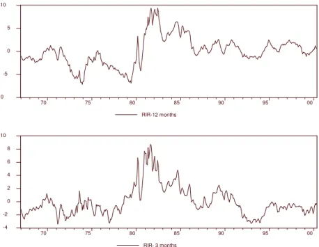
In this section, we investigate the presence of local persistency in economic time series. Since information on the dynamic of the shocks affecting the real side of the economy is very important to policy makers,we pay particular attention to three main real variables of the US economy: real exchange rate (RER), real interest rate (RIR) and real GNP
(RGNP). In other words, we want to investigate whetherthe effects of shocks on these
variables die out slowly (local persistence process), rapidly (ergodic stationary process) or never dissipate (near integrated or unit root process).
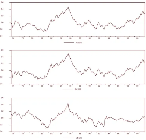
(RER(Fra-US)) Germany-USA (RER(Ger-(RER(Fra-US)), and the United Kingdom and the United States (RER(UK-US)). The data on the nominal exchange rate (end of period) and price level (Consumer Price Index) are collected from the International Financial Statistics CD-Rom, which is made by the International Monetary Fund (IMF). The sample covers the Post-Bretton Woods period that runs from April 1973 to March 2001, which totalizes 336 observations. Real exchange rates are in logarithm form.
The data on RGNP were collected from the U.S. Department of Commerce, Bureau of Economic Analysis. The data are measured in billions of fixed 1996 Dollars and are seasonally adjusted annual values, with first observation corresponding to the first quarter of 1967, which totalizes 141 observations. As with RER, RGNP is in logarithm form. As for the real interest rate, we used the nominal interest rate with 12-month and 3-month maturity together with the 12-month and 3-month ex-post in ation rates to calculate the real interest rates with 12-month (RIR-12m) and 3-month (RIR-3m) maturity. All the four series are monthly observed with first observation corresponding
to the first month of 1967, which totalizes 401 observations8. The timing of the data
is as follows: A January interest rate uses the end-of-January -month bill rate data.
A monthly observation of the -month in ation is calculated taking into account
observations ahead. For example, A January observation of the -month in ation rate
in the year is calculated from the January CPI data in the year to the January CPI
data in the year
Figures 1, 2 and 3 show graphs of RER, RIR and RGNP. The series of RER and RIR are centered with respect to their sample means whereas RGNP is showed in detrended values. One can see that all the variables display wide uctuations, but there seems to be a mean (trend) reversion in all cases. Therefore, we could expect unit root test to reject the null hypothesis of a unit root for these cases.
However, as suggested by past studies, this visual impression of mean reversion (or trend reversion) has been hard to establish statistically using traditional unit root
tests. Table VII shows the results of the ADF test9. Unlike the visual evidence, we
cannot reject the unit root hypothesis at 5% level of significance for the series of real exchange rate and real interest rate. Table VIII also show that the ADF test rejects the null hypothesis of unit root for the series of RGNP, which seems to suggest that the RGNP is trend stationary (TS). Trend stationarity of the RGNP has been previously reported in the literature by Diebold and Senhadji (1996) and Cheung and Chinn (1997).
CPI: We have used CPI data- all urbans and non-seasonally adjusted index - collected from Board of Governors of the Federal Reserve System, http://www.stls.frb.org/fred/
Three-month and twelve-month Treasury Bill Rate: Board of Governors of the Federal Reserve System, http://www.stls.frb.org/fred/
-0.4 -0.2 0.0 0.2 0.4 0.6
74 76 78 80 82 84 86 88 90 92 94 96 98 00
Fra-US
-0.4 -0.2 0.0 0.2 0.4 0.6
74 76 78 80 82 84 86 88 90 92 94 96 98 00
Ger-US
-0.4 -0.2 0.0 0.2 0.4 0.6
74 76 78 80 82 84 86 88 90 92 94 96 98 00
UK-US
-10 -5
0 5 10
70 75 80 85 90 95 00
RIR-12 months
-4 -2 0 2 4 6 8 10
70 75 80 85 90 95 00
RIR- 3 months
Figure 2: Real Interest Rates (centered)
-0.08 -0.06 -0.04 -0.02 0.00 0.02 0.04 0.06
70 75 80 85 90 95 00
RGNP
Nonetheless, it is important to mention that the rejection of the null hypothesis of unit root does not necessarily imply that the process is ergodic stationary, for instance, it can also be locally persistent.
Another interesting aspect displayed in Table VII is that most of the series have roots near unity and, as documented by Campbell and Perron (1991) and Dejong et. al. (1992), near unity roots may explain the failure to reject the unit root null in the ADF test . Since processes with high degree of local persistence have roots too close to unity, we should employ a more powerful test to reject the null hypothesis of unit root. Elliot et al (1996) introduced a modified unit root test (DF-GLS) that has better power when the AR coefficient is close to unity. Table VII shows the results from the DF-GLS test with the notation ’*’, ’**’, and ’***’ indicating that the null of unit root is rejected at 10%, 5% and 1% level of significance. By using the DF-GLS test, we reject the null hypothesis of unit root for all variables of our sample.
Table VII: Unit Root Tests
Series Specification Lags ADF DF-GLS
RER (Fra-US) Intercept 5 -1.85 0.98 -1.84**
RER (Ger-US) Intercept 8 -1.77 0.99 -1.74**
RER (UK-US) Intercept 6 -2.45 0.98 -1.89**
RIR-3m Intercept 8 -2.65* 0.97 -2.04**
RIR-12m Intercept 9 -2.13 0.98 -2.44**
RGNP Trend 4 -4.24** 0.96 -2.95**
In order to know whether the shocks die out slowly or rapidly, we recall that re-jecting the null of unit root does not imply to say that the process is ergodic stationary. For example, if a time series display local persistence, then the impulse response will converge to zero, but the shocks will take more time to die out. For this reason, we test covariance stationarity of these series.
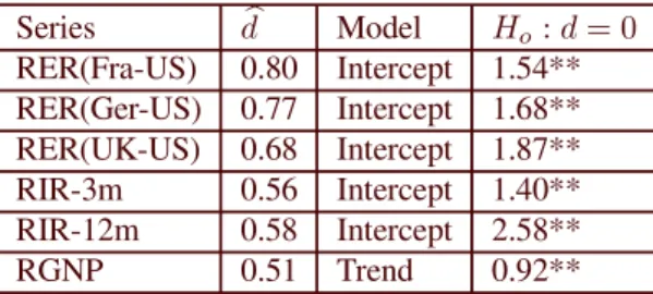
Table VIII reports the results for test of the null" against the alternative
" as well as point estimates of the local persistence parameter, .
We used the sample dependent truncation-lag- , where signifies an integer
number. Again, the notation ’*’, ’**’, and ’***’ suggest that the null hypothesis, is rejected at 10%, 5% and 1% level of significance, respectively. First, we notice that the results reported in Table X indicate that the data uniformly reject the stationarity
null hypothesis, i.e. against the alternative . In addition, all the series
have an estimated local persistence parameter, different from zero. Combining this
Table VIII: Results from Local Persistency Analysis
Series Model "
RER(Fra-US) 0.80 Intercept 1.54**
RER(Ger-US) 0.77 Intercept 1.68**
RER(UK-US) 0.68 Intercept 1.87**
RIR-3m 0.56 Intercept 1.40**
RIR-12m 0.58 Intercept 2.58**
RGNP 0.51 Trend 0.92**
6
Conclusion
We study local persistency of macroeconomic time series. To capture the dynamic of locally persistency time series, we use a block local to unity model. We have proposed statistical tests for the null hypothesis of stationarity (or trend stationarity) against local persistency. The test statistics converge to nonstandard limiting distributions that are functions of Brownian motions, involving higher order Brownian bridges. Tables of critical values are provided based on the asymptotic null distributions and a Monte Carlo experiment was conducted to examine the finite performance of these test, with special emphasis to the study of the finite sample size and power. The test is applied to several important variables of the US economy: real GNP, real interest rates, and real exchange rates. Our results suggest that these macroeconomic time series may be locally persistent and, therefore, display a pattern of temporal dependence that is different from the one generated by a traditional unit root and fractionally integrated process.
7
Appendix
Theorems 1 and 2 are properties under the stationarity null and are proven as in Xiao (1999).
Proof of Theorem 3.
For the estimation of) we consider the estimator
) . /
where. / It is well known that under" . /
and consequently) - Under" it can verified that
Thus,
. Given that- we get a
consis-tent test, that is,( as
[1] Beaudry, P. and Koop, G. (1993). ”Do recessions permanently change output?”,
Journal of Monetary Economics, 31: 149-63.
[2] Campbell, J.Y. and Perron, P. (1991). ”Pitfalls and Opportunities: What
NBER Economic Manual, Cambridge, MA.
[3] Cheung, Y-W. and Chinn, M.D. (1997). ”Further investigation on the uncertainty
unit root in GNP”. Journal of Business and Economic Statistics, 15: 68-73.
[4] Cheung, Y-W. and Lai, K. S. (1998). ”Parity reversion in real exchange rates during
the post-bretton woods period.” Journal of International Money and Finance,17: 597-614.
[5] ___________________. (2000). ”On cross-country differences in the persistence
of real exchange rates”. Journal of International Economics, 50: 375-97.
[6] ___________________. (2001). ”Long memory and nonlinear mean reversion in
Japanese yen-based real exchange rates.” Journal of International Money and Fi-nance.
[7] Cochrane, J. H. (1988). ”How big is the random walk in GNP? Journal of Political
Economy, 96: 893-920.
[8] Dejong, D.N., Nankervis, J.C., Savins, N.E. and Whiteman, C.H. (1992). ”The
power problem of unit root tests in time series with autoregressive errors.” Journal of Econometrics, 53: 323-43.
[9] Diebold, F. X. and Senhadji, A. S. (1996). ”The uncertainty root in real GNP:
Comment.” American Economic Review, 86: 1291-8.
[10] Dutkowsky, D. H. and McCoskey, S. K. (2001). Near integration, bank reluctance, and discount window borrowing. Journal of Banking and Finance 25: 1013-36.
[11] Elliott, G., Rothenberg, T.J. and Stock, J.H. (1996). ”Efficient tests for an autore-gressive unit root.” Econometrica, 64: 813-36.
[12] Feller, W. (1951). ”The asymptotic distribution of the range of sums of indepen-dent random variables.” Annals of Mathematical Statistics, 22: 427-32.
[14] Koenker, R. and Xiao, Z. (2002). ”Unit root quantile autoregression.” working paper, University of Illinois at Urbana-Champaign.
[15] Lanne, M. (2000). ”Near unit roots, cointegration, and the term structure of interest rates.” Journal of Applied Econometrics,15: 513-29.
[16] Lima, L.R., Xiao, Z. (2002). ” Co-movement of locally persistent processes.” working paper, University of Illinois at Urbana-Champaign.
[17] Perron, P. and Ng, Serena. (2001). ”Lag length selection and the construction of unit root tests with good size and power.” Econometrica, 69: 1519-54.
[18] Phillips, P.C., Moon, H.R. and Xiao, Z. (2001).” How to estimate autoregressive roots near unity.” Econometric Theory 17, 29-69.
[19] Ploberger, W., Kramer, W. and Kontrus, K. (1989). ”A new test for structural sta-bility in the linear regression model.” Journal of Econometrics 40: 307-18.
[20] Protter, P. (1990). ”Stochastic integration and differential equation.” Springer, New York.
[21] Xiao, Z. (1999): ”A Residual based test for the null hypothesis of cointegration.” Economics Letters, 64, 133-141.