Carlos De Marqui Junior
Engineering School of Sao Carlos University of Sao Paulo Laboratory of Aeroelasticity Flight Dynamics and Control Av. Trabalhador Sancarlense 400 13566- 590 Sao Carlos, SP. Brazil [email protected]
Daniela C. Rebolho
Eduardo M. Belo
and Flávio D. Marques
Identification of Flutter Parameters for
a Wing Model
A flexible mounting system has been developed for flutter tests with rigid wings in wind tunnel. The two-degree-of-freedom flutter obtained with this experimental system can be described as the combination of structural bending and torsion vibration modes. Active control schemes for flutter suppression, using a trailing edge flap as actuator, can be tested using this experimental setup. Previously to the development of the control scheme, dynamic and aeroelastic characteristics of the system must be investigated. Experimental modal analysis is performed and modes shape and frequencies are determined. Then, wind tunnel tests are performed to characterize the flutter phenomenon, determining critical flutter speed and frequency. Frequency response functions are also obtained for the range of velocities below the critical one showing the evolution of pitch and plunge modes and the coupling tendency with increasing velocity. Pitch and plunge data obtained in the time domain during these tests are used to evaluate the ability of the Extended Eigensystem Realization Algorithm to identify flutter parameter with increasing velocity. The results of the identification process are demonstrated in terms of the evolution of frequency and damping of the modes involved in flutter.
Keywords: Identification, flutter, EERA, aeroelasticity
Introduction
Aeroelastic phenomena result from the interaction of elastic, inertial, and aerodynamic loads on aeronautical structures. When elastic bodies are exposed to airstream, structural deformations induce additional aerodynamic forces and these forces produce additional structural deformations, which again will induce greater aerodynamic forces. This interaction may lead to aeroelastic instabilities such as flutter, for example see Försching (1979). After World War II the increase in flight speed and structural modifications made aeroelastic problems more significant. The changes and historical evolution of aeroelasticity through out the history are described in Ashley (1970), Collar (1959), Garrick and
Reed (1981), and Garrick (1976).1
Flutter is one of the most representative topics of aeroelasticity. Flutter is a complex phenomenon where structural modes are simultaneously coupled and excited by aerodynamic loads. In a more formal way, flutter is the condition where an aircraft component exhibits a self-sustained oscillatory behaviour at speeds higher than the critical one (Wright, 1991). In general, flutter occurs on lifting surfaces submitted to large aerodynamic loads, such as wings and tails.
Flight flutter testing (Kehoe, 1995) is a very important part in the certification of an aircraft. During these time consuming and high cost tests the flight envelope must be expanded safely in order to show that the aircraft is flutter free throughout the desired conditions. The procedure is made up of three stages (Cooper and Crowther, 1999):
1 The aircraft is excited in some manner and responses are
measured at some speed;
2 Flutter parameters are estimated using system identification
methods;
3 A decision is made to proceed to the next flight test point or not. The main task of these flight tests is to predict stability at the next test speed with confidence, allowed by estimating aeroelastic parameters (stage two). The development of methods to accurately predict the speed related to the flutter onset from the measured test data, or any other aeroelastic instability, is an important way to
Presented at XI DINAME – International Symposium on Dynamic Problems of Mechanics, February 28th - March 4th, 2005, Ouro Preto. MG. Brazil. Paper accepted: June, 2005. Technical Editor: José Roberto de França Arruda.
increase the safety and even to reduce costs of these tests (Lind, 2003). Several methods have been developed in order to achieve this objective. In general, these methods are developed and tested using data from simulations, but evaluations which include data from flight testing must be done before an approach can reliably be used for an envelope expansion.
Some methods have been shown to be theoretically valid to predict flutter speeds, for instance, those on extrapolating damping trends as described by Kehoe (1995). The envelope function developed by Cooper; Emmett and Wright (1993) is another method. This function is based on the assumption that the impulse response function contains information about the overall stability of the system. Similarly, a discrete-time autoregressive moving average model (ARMA) uses the Jury Stability criterion and also considers the overall stability of the system (Torii and Matsuzaki, 2001). Another method is the Zimmerman-Weissenburger flutter margin method, where the Routh stability criterion should be used instead of a damping tracking (Zimmerman and Weissenburger, 1964). The flutterometer is an on-line model-based tool used to predict flutter margins developed by Lind and Brenner (2000). This tool uses experimental data and theoretical models to predict the flutter onset.
The ability of the aforementioned methods to predict flutter parameters from flight tests is evaluated by Lind (2003). The flight tests were performed using a F-15 as a host carrier for an aerostructure test wing (ATW). This ATW is not a complete aircraft, but it is a realistic wing and the envelope could be expanded during the flight tests to a point at which its flutter speed would be achieved. As the true flutter speed is known, it can be used to evaluate the predicted flutter speeds. The results obtained from these evaluations indicate the strengths and weaknesses of each method in different conditions. For example, the data-based methods are unable to predict flutter speed accurately using data from low-speed tests, but converge to a good solution as the airspeed is increased. However, the model-based flutterometer is conservative using data from low-speed tests, but predictions remain conservative and do not converge to the true flutter speed using data from high-speed tests. These facts suggest that a more efficient flight-test program for envelope expansion could be formulated with the combination of various identification approaches.
wind tunnel tests. The wind tunnel tests are performed with a flexible mounting system designed to the achievement of two-degree-of-freedom flutter when associated with a rigid wing model. The wind-off characteristics and aeroelastic characteristics of this experimental system have been extensively determined through finite element simulations, experimental modal analysis and wind tunnel tests (De Marqui Jr et al., 2004). Thus, this well-known experimental system can be used to predict flutter velocity using the EERA method.
The EERA method is a modified form of a Eigensystem Realization Algorithm (ERA), which is a time domain algorithm that can indentify the modes simultaneously (Juang, 1994). The EERA calculates the modal parameters by manipulating the block Hankel matrices from both input and output time histories (Tasker; Bosse and Fisher, 1998). The development of these subspace identification methods is motivated by difficulties in estimating modal parameters for multiple-input multiple-output vibratory systems. During the last few years subspace methods have attracted attention in the field of system identification, because they are essentially non-iterative and fast (Favoreel et al., 1999). Therefore, no convergence problems arise and since the subspace methods are only based on stable techniques of linear algebra, they are also numerically robust. These methods accomplish substantial filtering of the data using eigenvalue or singular value decomposition and are particularly effective when there are closely spaced modes. In essence, the data are separated into orthogonal signal and null subspaces, either of which may be used to estimate the modal parameters (Tasker; Bosse and Fisher, 1998).
Nomenclature
m = number of output
n = degree of freedom
r = number of external excitations
k = sample instant
M =number of samples in a time window
N = number of samples in a time window
u(k) = input vector
x(k) = state vector
y(k) =response vector
Ad= system matrix Bd= input matrix Cd= output matrix
Dd= direct transmission matrix
G= block Toeplitz matrix
I = identity matrix
R= matrix of the left singular vectors
S= matrix of the right singular vectors
U= block Hankel matrices of inputs
X= matrix of the state sequence
Y= block Hankel matrices of outputs
0= null matrix
Greek Symbols
ΓΓΓΓ = extended observability matrix
∑ ∑ ∑
∑= matrix of singular values
Subscripts s shifted
2n first 2n columns
Superscripts
-1 inverse
T transpose orthogonal † pseudoinverse
Physical Model
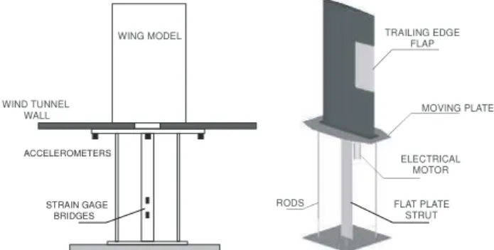
The physical model is a rigid rectangular wing with a NACA 0012 airfoil section associated with a flexible mounting system. The flexible mounting system provides a well-defined two-degree-of-freedom dynamic system in which the rigid wing will encounter flutter. Side and perspective views of the flutter mounting system are presented in Fig. 1. The flutter mounting system consists of a moving plate supported by a system of four circular rods and a centred flat-plate strut, similar to the system developed in Dansberry
et al. (1993).
The rods and the flat-plate provide the elastic constraints and the rigid wing model fixed in the moving plate will oscillate in a two-degree-of-freedom mode, that is, pitch and plunge, when flutter is encountered. The rods, flat-plate and moving plate are made of steel and all connections are fixed-fixed end. The wing model and the moving plate are made of aluminum and the trailing edge flap is made of ABS resin. Their dimensions are: rods 0.0055 m in diameter; moving plate is 0.6 × 0.3 m; flat-plate is 0.7 × 0.1 × 0.002
m and the wing model has 0.8 × 0.45 m. The trailing edge flap ranges from 37.5 % to 62.5 % of the wingspan and its chord is 35 % of the full wing chord.
WING MODEL
WIND TUNNEL
WALL MOVING PLATE
RODS FLAT PLATE
STRUT TRAILING EDGE
FLAP
ELECTRICAL MOTOR
STRAIN GAGE BRIDGES ACCELEROMETERS
Figure 1. Side and perspective views of the flutter mounting system.
The wind-off characteristics of the flutter mounting system are strongly influenced by the dimensions of the flat-plate strut, the rods and the mass of the moving plate and wing model. Modifications in the length and cross section of the flat plate strut and rods modify the frequencies and mode shapes of the flexible mounting system. Weights can be added to decouple the pitch and plunge modes by moving the centre of gravity of the flexible mounting and wing model to the system elastic axis. The system elastic axis is located in the vertical centreline of the flat plate strut and centre of the moving plate. The four rods also assure a parallel pitch and plunge displacement relative to the wind tunnel wall.
To design the flexible system, a Finite Element Model was developed using the software Ansysâ. Two types of elements were used: Beam 4 and Shell 63, for the rods and flat plate strut, respectively. The cantilever boundary condition was adopted for the flexible mount system at the rods and flat plate strut base. The dimensions and dynamic characteristics of the experimental system obtained from the FEM were modified until the aeroelastic behaviour of this system could be adjusted to the available wind tunnel. The aeroelastic behaviour of this system was simulated with a mathematical model described in De Marqui Jr, Belo and Marques (2005).
flat-plate strut, because it provides the elastic constraints to the system. The Eigensystem Realization Algorithm (ERA) modified by Tsunaki (1999) is employed to identify the mode shapes and frequencies from the experimental data. The most significant natural frequencies are listed in Tab. 1. Rods and chordwise modes were not investigated in this modal analysis.
Table 1 shows first bending and first torsion modes well defined and it also shows the third mode higher than those. Theoretically, this condition assures a two-degree-of-freedom system during the wind tunnel tests, higher modes will not be significantly excited during wind tunnel tests (Dansberry et al., 1993). Details on the flexible mounting system design procedure and more results can be found in De Marqui Jr et al. (2004).
The modal analysis takes into account only the structural aspects of the flutter problem. Obviously the interaction of these characteristics with the aerodynamic ones has to be considered in the flutter analysis. Aerodynamic forces and moments, lift and pitch moment in the case of this study, will be exciting the modes involved in the classical bending-torsion flutter. As a consequence, the elastic characteristics of the structure and the resulting aerodynamic restoring loads, responsible for aerodynamic damping when no mechanical friction is assumed and caused by the upwash induced by the wake vortices, will be reacting and dissipating energy to the airstream. When the critical speed is achieved, the aerodynamic damping vanishes because the aerodynamic restoring forces loose their dissipative characteristics and the self-sustained oscillatory behaviour is verified.
Table 1. Some properties of the most significant modes.
Mode Description Frequency
(Hz) Damping Stiffness
1 First bending (plunge) 1.2 0.04 1290 N/m 2 First torsion (pitch) 2.4 0.02 Nm/rad 44
3 Second bending 11.7 --- ---
The experimental system, wing associated with the mounting system, is instrumented with two strain gauges and three accelerometers, as it can be seen in Fig 1. One accelerometer (Kistler KBeam 8303A10M4) is placed in the centre line of the flat plate strut measuring the plunge acceleration. Other two accelerometers (Kistler KBeam 8304B10) are installed in the moving plate. The signals measured with these accelerometers are used to calculate the pitch acceleration.
The strain gauges are located in the centreline of the flat plate strut in a maximum strain position determined from the finite element analyses. One strain gauge (Kiowa KFG-5120C123) is calibrated to measure plunge displacements and the other (Kiowa KFC-2D211) is calibrated to measure pitch angles.
A brushless electrical motor (Thompson BLD–2315B10200) installed in the lower surface of the moving plate (cf. Fig. 1) is used to drive the trailing edge flap. The flap is connected to the motor by a shaft. The electrical motor has an encoder that is used to measure the actual angular position of the flap. A PID controller was tuned to assure the correct control of the trailing edge flap position by the motor.
Extended Eigensystem Realization Algorithm - EERA
Any linear time-invariant dynamic system with n degree-of-freedom can be modelled by the following discrete time state space equations:
(
)
( )
( )
( )
k( )
k( )
kk k k d d d d u D x C y u B x A x + = + = +1
, (1)
where x(k) is the 2n dimensional state vector at the kth sample
instant, u(k) is the r dimensional input vector, r is the number of external excitations, y(k) is the m dimensional response vector, m is the number of output or response of the system, Ad is the 2n × 2n
system matrix, Bd is the 2n×r input matrix, Cd is the m×2n output matrix, and Dd is the m×r direct transmission matrix.
The identification procedure using the EERA consists in the determination of the system matrix Ad from the inputs and outputs
time history. Features related to flutter, namely frequencies and
damping, can be estimated using the system matrix Ad. The
identification of the system matrix Ad using the EERA method is described by the following procedure based on the theory presented by Tasker; Bosse and Fischer (1998).
The block Hankel matrices of inputs (U) and outputs (Y) can be obtained directly from the input and output time (Overschee and De Moor, 1996)
( )
( )
(
)
( )
( )
( )
(
) (
)
(
)
(
M)
( )
M(
M N)
rM N N M M M N N × − + − − + − − − = 2 1 3 1 2 2 1 1 1 0 u u u u u u u u u u u u U ⋯ ⋯ ⋮ ⋮ ⋮ ⋮ ⋯ ⋯ , and( )
( )
(
)
( )
( )
( )
(
) (
)
(
)
(
M)
( )
M(
M N)
mM NN M M M N N × − + − − + − − − = 2 1 3 1 2 2 1 1 1 0 y y y y y y y y y y y y Y ⋯ ⋯ ⋮ ⋮ ⋮ ⋮ ⋯ ⋯ (2)
where, M and N are the number of samples in a time window that will be used during the identification process.
One can verify that the block Hankel matrix of outputs are represented as described in Verhaegen and Dewilde (1992),
U G X
Y=Γ + (3)
where ΓΓΓΓ is an extended observability matrix, Xis a matrix of the state sequence, and G is a block Toeplitz matrix of Markov parameters or impulse response, that is.,
n mM M d d d d d d d A C A C A C C 2 1 2 × − = ⋮
Γ ,X=
[
x( ) ( )
1 x2 ⋯ x( )
N]
2n×NandrM mM d d M d d d M d d d d d d d d d d d × − − = D B A C B A C 0 B C B A C 0 D B C 0 0 D G ⋯ ⋮ ⋮ ⋮ ⋮ ⋯ ⋯ ⋯ 3 2 (4)
By definition, the orthogonal matrix can be written as (Van Overschee and De Moor, 1996),
(
UU)
U UI
Post-multiplying Eq. (3) by the right and left terms of Eq. (5), respectively, and using the definition of orthogonality, the following expression can be obtained,
⊥ ⊥=
U X U
Y Γ . (6)
Applying the singular value decomposition to YU⊥:
T
S R U
Y ⊥= Σ , (7)
where R (mM × mM) is the left singular vectors matrix, Σare the corresponding singular values matrix and S (N × N) is the right singular vectors matrix. The columns of these matrices are orthonormal.
The pseudoinverse of YU⊥ can be obtained from Eq.(7) given:
( )
YU † SΣ†RT=
⊥ , (8)
while,
(
YU)
ImMU
Y ⊥ ⊥†= , and
(
YU)
YU =IN⊥ ⊥†
. (9)
At this point, a shifted form of the block Hankel matrix of the output, or response, can be introduced as:
( )
( )
( )
( )
(
)
(
)
( )
(
)
(
)
(
)
mM Ns N M M ) M ( N M M M N N ) ( × − + + − + − + = 1 1 2 1 1 3 2 2 1 y y y y y y y y y y y y Y ⋯ ⋯ ⋮ ⋮ ⋮ ⋮ ⋯ ⋯
. (10)
The dimensions of this new matrix are connected to the length of output time history vector (number of samples in a time window) that will be used during the identification process. However, this window must be advanced one or more steps in time.
In way similar to the Eq. (3), it follows:
U G X
Ys=Γs + s , (11)
where ΓΓΓΓs and Gs are shifted versions of extended observability
matrix and block Toeplitz matrix of Markov parameters, respectively: n mM M d d d d d d d d s 2 3 2 × = A C A C A C A C ⋮ Γ ,and rM mM d d M d d d M d d d d d d d d d d d d d d d d s × − − = D B A C B A C 0 B A C B A C 0 B C B A C 0 D B C G ⋯ ⋮ ⋮ ⋮ ⋮ ⋯ ⋯ ⋯ 2 1
2 . (12)
Following the same derivation used for Eq. (6), it is then possible to obtain:
⊥ ⊥ ⊥= = XU A XU U
Ys Γs Γ d , (13)
where, the term on the right side of this equation is easily obtained comparing the original and shifted versions of the observability matrices, that is, ΓΓΓΓs = ΓΓΓΓAd.
The matrix YsU⊥⊥⊥⊥ from Eq. (13) can be conveniently rewritten
as,
(
⊥)( )
⊥ ⊥( ) ( )
⊥ ⊥ ⊥= U Y U Y U Y U Y U Y UYs † s † . (14)
Substituting Eq. (7) and Eq. (8) in Eq. (14), results
(
)(
)
(
T)(
T)
s T T
sU R S S R Y U S R R S
Y ⊥= Σ Σ−1 ⊥ Σ−1 Σ (15)
At this stage, a criterion to determine the number of necessary singular values can be stipulated. This number can be modified according to the difficulties involved in the identification process. This number will establish the dimension of the identified model and it must be modified during the identification problem. Considering that the number of singular values is determined as 2n, the singular values matrix can be represented as:
[
n]
n diag 1, 2, , 2
2 σ σ σ
Σ = …
with
0
2 2
1≥σ ≥ ≥σ n≥
σ … (16)
The, the matrices can be conveniently written as
= 0 0 0 n 2 Σ Σ ,
[
R2 R0]
R= n ,
[
]
Tn T
0 2 S
S
S = , (17)
where, R2n contains the first 2n columns of R and S2n contains the
first 2n columns of S.
The matrices R2n and S2n satisfy the following relation:
n T
n n T
n 2 2 2
2R I S S
R = = . (18)
By using the relations in Eq. (17) to the singular value decomposition problem, it results:
[
]
Tn n n T T n n n T 2 2 2 0 2 2 0
2 R S
S S 0 0 0 R R S
RΣ Σ = Σ
= , (19)
and, if ΣΣΣΣ†=ΣΣΣΣ-1 (Watkins, 1991), it follows:
(
) (
)
Tn n n T n n n T T 2 1 2 2 † 2 2 2 † † R S S R S R R
SΣ = Σ = Σ = Σ− . (20)
Considering that 2 1 2n 2 1 2n 1 2n Σ Σ
Σ − − −
= . (21)
and substituting Eq. (19) and Eq. (20) in Eq. (15)
(
)
(
T)
n n n T n / n / n n T n n n
s 2 2 2 2
2 1 2 2 1 2 2 2 2
2 S S R R S
R U
Y ⊥= Σ Σ− ΞΣ− Σ (22)
where 2 1 2 2 2 2 1 2 / n n s T n / n − ⊥ −
=Σ Σ
From Eq. (18), it follows:
T n / n / n n s T
n / n / n n
s 2
2 1 2 2 1 2 2 2
2 1 2 2 1 2
2 R Y U S S
R U
Y ⊥= Σ Σ− ⊥ Σ− Σ . (24)
Equation (24) can be compared with Eq. (13) and, then, the system matrix can be assessed as follows:
2 1 2 2 2 2 1 2
/ n n s T
n / n d
− ⊥ −
=Σ R Y U S Σ
A . (25)
The system matrix Ad is a minimum realization of the system. The dimension of this matrix is 2n and it also determines the dimension of the identified system. This realization can be transformed to state equations in modal coordinates and natural frequencies and damping can be obtained by calculating the eigenvalues. The above expression differs from the ERA expression only by the presence of the input term. When the responses are due to impulsive inputs, the expression is identical to the expressions observed in ERA (Juang, 1994).
Experimental Flutter Verification
A dSPACE DS 1103 processor board is used to develop the real time control of the flap and for data acquisition. This board has a 400 MHz Power PC 604e processor, I/O interfaces with 16 A/D
and 8 D/A channels and incremental encoder interface (DSPACE,
2001). The signals of the accelerometers, strain gauge bridges and flap position can be acquired simultaneously. The computational codes for data acquisition and signal processing are developed in Matlab/Simulink. The Simulink code is compiled in Matlab
using Real-Time Workshop compiler resulting in a C code. This C
code is downloaded to the dSPACE board to perform signal
processing and I/O control.
Figure 2 shows a simplified scheme of the data acquisition system. The gains in the computational system are used to convert the measured signals to the necessary physical units, mV to m/s2 or rad/s2 for the accelerometers and mV to m or rad for the strain gauges. The encoder of the electrical motor used to drive the trailing edge flap has 1000 lines. Therefore, a resolution of 0.36 degrees can be achieved in the measurements of the trailing edge position. During the experiments, an acquisition rate of 1000 samples per second is employed.
Encoder
A/D Pitch strain
gauge bridge
Plunge strain gauge bridge
Pitch acceleromenters
Plunge acceleromenter
A/D
A/D
A/D Nexus
B&K HBM MGCPlus
Enc
Gain 1
Gain 2
Gain 3
Gain 4
Gain 5
Disk
Figure 2. Simplified scheme of the data acquisition system.
In the first experimental test, the verification of the critical flutter velocity is performed. The wind tunnel velocity is gradually increased and the pitch and plunge signals measured using the dSPACE system. The wind tunnel velocity is obtained from the pressure measurements performed with a static pitot tube associated with a Betz manometer, a barometer and a temperature sensor
installed on the test chamber. Flutter is observed at the critical flow velocity of 25 m/s, when the oscillatory behaviour is measured. Figure 3 presents the pitch and plunge signals, respectively, measured during the experiments.
0 5 10 15
-0.4 -0.2 0 0.2 0.4 0.6
Time (s)
P
lu
n
g
e
(
m
/s
)
0 5 10 15
-1 -0.5 0 0.5 1
Time (s)
P
itc
h
(
ra
d/
s)
Figure 3. Pitch and plunge responses measured during wind tunnel tests at critical flutter velocity.
One of the characteristics of the flutter phenomenon is the coupling of the modes involved in the phenomenon i.e., pitch and plunge in the case. This condition is verified in Fig. 4, where the time domain signals presented in Fig. 3 are presented in terms of their frequency content.
0 1 2 3 4 5
0 0.2 0.4 0.6 0.8 1
Frequency (Hz)
F
F
T
(
pi
tc
h
a
nd
p
lu
n
ge
) Plunge
Pitch
Figure 4. Frequency domain representation of pitch and plunge responses obtained during wind tunnel tests at critical flutter velocity.
This test shows the system behaviour only at the critical velocity. But some dynamical characteristics change with increasing wind tunnel flow velocity. In order to verify these changes other tests are performed. Basically, frequency response functions are obtained in several velocities showing the evolution of first bending and torsion modes with increasing speed. The input signal considered during these tests is the trailing edge position and the output signal is the acceleration measured in the wing trailing edge.
analyser. This procedure is repeated for all intermediate test velocities.
In Fig. 5, one can verify the evolution of the modes with increasing wind tunnel velocity. The frequency response obtained at zero velocity presents peaks relative to first bending and torsion modes well-defined and the same natural frequencies obtained during the EMA, as expected. In the last frequency response, measured near to the critical velocity, one can verify the tendency of coupling between the modes involved in flutter. This coupling tends to occur at frequency about 1.6 Hz, confirming the result observed in Fig. 4.
In the frequency responses obtained in intermediate velocities, the variations in pitch and plunge frequencies can be observed. Also, it is clear that the peaks of pitch and plunge modes are not so sharp as the peaks of the frequency response at zero velocity. This fact can be seen as the effect of fluid structure interaction on damping increase. This tendency is expected until velocities near the critical one, when the damping is expected to vanish and flutter occurs.
0 1 2 3 4 5 6 7
0 5 10 15 20 25 -80 -60 -40
Frequency (Hz) Velocity (m/s)
d
B
(
m
/s
2
/
d
eg
re
e
)
Figure 5. Frequency responses obtained in several velocities during wind tunnel tests.
Identification Results
The Extended Eigensystem Realization Algorithm (EERA) is employed to quantify the variation of frequencies and damping values with wind tunnel increasing velocity relative to the modes involved in flutter. By inspecting the damping evolution with airspeed variation using EERA one can predict when flutter is expected to occur. The data used in the identification process are acquired during the aeroelastic tests performed to obtain the frequency response function previously described in this paper. Simultaneously to the frequency domain tests, the input signal (trailing edge flap motion) and the signal measured by the strain gauges (pitch and plunge displacements) were captured in time
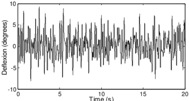
domain using the dSPACE® acquisition system. Figures 6 to 8 show
examples of input and output signals measured during one of the wind tunnel tests. In Fig. 6 the flap deflection in degrees is depicted. It represents a randomly generated (uniform distribution) signal to the flap angle in order to work as an excitation to the aeroelastic system. Both plunge and pitch responses, with respect to the flap motion (see Fig. 6), are shown in Figs. 7 and 8, respectively.
0 5 10 15 20
-10 -5 0 5 10
Time (s)
D
e
fle
xi
o
n
(
d
e
g
re
e
s)
Figure 6. Deflection of the flap (input signal) measured during the wind tunnel test.
0 5 10 15 20 25 30
-0.04 -0.02 0 0.02 0.04 0.06
Time (s)
P
lu
n
ge
(
m
)
Figure 7. Plunge (output signal) measured during the wind tunnel test.
0 5 10 15 20 25 30
-0.1 -0.05 0 0.05 0.1
Time (s)
P
itc
h
(
ra
d)
Figure 8. Pitch (output signal) measured during the wind tunnel test.
The identification process was performed after the acquisition of input and outputs time domain data. The dimensions of the block Hankel matrices of inputs and outputs (M and N=2M) and the number of singular values (2n) to be considered were modified for each identification performed for each flow velocity. This variation can be explained by the difficulties involved in the identification of parameters using data acquired at higher wind tunnel velocities, when modes are getting coupled.
for a variety of identification parameters. Nonetheless, for the damping factor identification the values per airspeed were more disperse. The damping values for pitch mode seems lesser disperse than those for plunge mode. The reasons for that are still not determined, and it must be object for ongoing investigation on flutter prediction with EERA. Although these results may be poorer than those for the frequency, the average damping values show curves that are consistent with the physics of the classical 2D flutter. While pitch (torsion) mode leads to flutter, the plunge (bending) mode goes towards over-damping.
1 1.5 2 2.5 3
First bending (plunge) First torsion (pitch)
F
re
q
u
e
n
c
y
(
H
z
)
0 5 10 15 20 25 30
0 2 4 6 8 10
D
a
m
p
im
g
F
a
c
to
r
(
%
)
Velocity (m/s)
Figure.9 Flutter parameters identified using EERA and data from wind tunnel tests.
Conclusions
The experimental aeroelastic test in wind tunnel has been used for the identification of flutter parameters. Wind tunnel tests have been performed for flutter characterization and the phenomenon could be observed in the time and frequency domains. In the time domain results the self-sustained oscillatory behaviour of flutter was shown. In the frequency domain responses the evolution of the modes with wind tunnel increasing velocity was also observed. At the critical velocity, the coupling tendency could be clearly demonstrated. The variations in pitch and plunge damping could be obtained just in a qualitative way in these tests.
In order to quantify the evolution of pitch and plunge modes with increasing velocity an identification method was applied. The Extended Eigensystem Realization Algorithm was employed using the input and output data obtained, in the time domain, during the tests performed for flutter characterization. This method was employed on the identification of flutter parameters in order to verify its performance in terms of velocity and possible numerical problems during the process. The use of EERA can be said to be appropriate considering the coherence between the results obtained with this identification method and the results obtained in previous wind tunnel tests. Some difficulties have occurred in the identification of damping factor values, in particular, for the plunge mode. Further investigations on why such problems occur are necessary, and are ongoing.
Even considering that the identification process presented in this work is an off-line one, the results obtained up to now indicate that the on-line identification of flutter parameters during wind tunnel tests can be explored. The development of an adaptive control system obtained with the association of the on-line identification method and a control law for flutter suppression can be achievable in further research.
Acknowledgements
The authors gratefully acknowledge the financial support provided by CAPES and FAPESP (Sao Paulo State Foundation for Research Support – Brazil) through contract numbers 1999/04980-0 and 2000/00390-3.
References
Ashley, H., 1970, “Aeroelasticity”, Applied Mechanics Reviews, pp.119-129.
Collar, A.R., 1959, “Aeroelasticity – Retrospect and Prospect”, The Journal of the Royal Aeronautical Society, Vol. 63, No. 577, pp.1-15, 1959.
Cooper, J.E. and Crowther, W.J., 1999, “Flutter Speed Prediction During Flight Testing Using Neural Networks”, CEAS/AIAA/ICASE/NASA Langley International Forum on Aeroelasticity and Structural Dynamics, pp. 255-264.
Cooper, J.E., Emmett, P.R. and Wright, J.R., 1993, “Envelope Function: A Tool for Analysing Flutter Data”, Journal of Aircraft, Vol. 30, No. 5, pp. 785-790.
Dansberry, B.E., Durham, M. H., Bennett, R. M., Turnock, D. L., Silva, E. A. and Rivera Jr, J. A., 1993, “Physical Properties of the Benchmark Models Program Supercritical Wing”, NASA TM-4457.
De Marqui Jr., C., Belo, E.M. and Marques, F.D., 2005, “A flutter suppression active controller”, Proc I.Mech.E Part G - Journal of Aerospace Engineering, Vol. 219.
De Marqui Jr., C., Belo, E.M., Tsunaki, R.H., Rebolho, D.C. and Marques, F.D., 2004, “Design and Tests of an Experimental Flutter Mount System”, Proceedings of the XXII IMAC, Dearborn, MI.
DS1103 PPC Controller Board, 2001, Hardware Reference, www.dspace.de.
Favoreel, W., Huffel, S.V., De Moor, B, Sima, V. and Verhaegen, M., 1999, “Comparative study between three subspace identification algorithms”, Proceedings of the European Control Conference, Karlsruhe-Germany, 31st August-3rd September, 6p.
Försching, H., 1979, “Aeroelastic Problems in Aircraft Desing”, von Karman Institute for Fluid Dynamics, Lecture series 08: A Survey of Aeroelastic Problems.
Garrick, I.E. and Reed, W.H., 1981, “Historical Development of Aircraft Flutter”, Journal of Aircraft, Vol.18, No. 11, pp. 897-912.
Garrick, I.E., 1976, “Aeroelasticity – frontiers and beyond”, 13th Von Karman Lecture, Journal of Aircraft, Vol.13, No. 9, pp. 641-657.
Juang, J.N., 1994, “Applied System Identification”, Prentice Hall PTR, New Jersey, USA.
Kehoe, M.W., 1995, “A Historical Overview of Flight Flutter Testing”, NASA TM-4720.
Ko, J., Kurdila, A.J. and Strganac, T.J., 1997, “Adaptive Feedback Linearization for the Control of a Typical Wing Section with Structural Nonlinearity”, ASME International Mechanical Engineering Congress and Exposition, Dallas, Texas.
Lind, R. and Brenner, M., 2000, “Flutterometer: An On-Line Tool to Predict Robust Flutter Margins”, Journal of Aircraft, Vol. 37, No. 6, pp. 1105-1112.
Lind, R., 2003, “Flight-Test Evaluation of Flutter Prediction Methods”,
Journal of Aircraft, Vol. 40, No. 5, pp. 964-970.
Mukhopadhyay, V., 1995, “Flutter suppression control law design and testing for the active flexible wing”, Journal of Aircraft, Vol.32, No. 1, pp 45-51.
Tasker, F., Bosse, A. and Fisher, S., 1998, “Real-time modal parameters estimation using subspace methods: Theory”. Mechanical Systems and Signal Processing, Vol.12, No. 6, pp. 797-808.
Torii, H. and Matsuzaki, Y., 2001, “Flutter Margin Evaluation for Discrete-Time Systems”, Journal of Aircraft, Vol. 38, No. 1, pp. 42-47.
Van Overschee, P. and De Moor, B., 1996, “Subspace identification for linear systems: theory, implementation, applications”, Kluwer Academic Publishers, Boston, United States.
Verhaegen, M. and Dewilde, P., 1992, “Subspace model identification part 1. The output-error state space model identification class of algorithms”,
International Journal of Control, Vol. 56, pp. 1187-1210.
Waszak, M.R., 1998, “Modeling the benchmark active control technology wind-tunnel model for active control design applications”, NASA TP-1998-206270.
Watkins, D.S., 1991, “Fundamental of Matrix Computations”, New York, Wiley,USA.
Wright, J.R., 1991, “Introduction to Flutter of Winged Aircraft”, von Karman Institute for Fluid Dynamics, Lecture series 01: Elementary Flutter Analysis.