A Simple Theory for Vibration of MRI Gradient Coils
D. Tomasi1 and T. Ernst2
1Medical Department, Brookhaven National Laboratory, Upton, NY, 11973 and 2Department of Medicine, Hawai University, Honolulu, HI, 96813
Received on 28 August, 2005; accepted on 28 November, 2005
Vibrations of a string can provide a model for vibrations of MRI coil assemblies. The string model for the vibrations of MRI coils is presented, and compared with experimental results. Gradient coils exhibit resonant modes because of the finite coil length,l, and the elasticity of materials that comprise the assembly. The reso-nance frequencies depend onland the Young modulus, as well as on the current distribution. Under longitudinal gradient pulses, anti-symmetrical modes of surface vibration are produced due to the symmetry of current distri-bution. In contrast, transverse gradient pulses produce coil bending that results in symmetrical vibration modes of the coil axis. The viscosity of the assembly materials controls the width of the vibrational resonance modes. Experimental results are in agreement with this simple string model.
Keywords: MRI; MRI coils
I. INTRODUCTION
The high-intensity acoustic noise produced by fast MRI techniques, such as echo-planar imaging (EPI), has been a concern for patient safety and comfort.The sound pressure level (SPL) of acoustic noise in MRI systems can exceed 100 dB, and may cause anxiety and discomfort in patients [1]. Acoustic noise can also obscure functional magnetic res-onance imaging (fMRI) studies. For instance, loud acoustic noise can produce spurious areas of activation in the auditory cortex [2-3] or alter the BOLD signal in motor and visual cor-tices [4-5]. Acoustic noise is a consequence of the vibrations produced in the coil assembly by the Lorentz interaction be-tween the static magnetic field, B0, and the time-dependent currents in gradient wires. The SPL of acoustic noise in MRI scanners is commonly reduced by the use of acoustic absorb-ing materials and ear protection (ear plugs and headphones). In addition, the SPL can be reduced by the development of “silent” MRI-pulse sequences [6-9] or the design of “quiet” gradient coils [10-13]. Several experimental studies [14-17] have demonstrated a clear increase in SPL of acoustic noise for high-field systems [14], and the existence of acoustic res-onances [15]. However, the vibrational motion of gradient assemblies, where the acoustic noise originates, has not been studied extensively. Therefore, we developed a simple model, based on the vibrations of an elastic string, to understand the vibration motion of gradient assemblies. Additionally, we measured the vibration motion of our gradient coil to test the model.
II. THEORY
Longitudinal gradients
Since MRI gradient coils are operated in magnetic fields, a Lorentz force acts on the coil wires during gradient current pulses. We assume that the main magnetic fieldB0is along the z-axis. For a current density,j(φ,z,t), on a cylindrical surface of radiusa, the magnetic force element,dF, is a radial vector
caused by theφ-component of the current density, jφ(φ,z,t): dF(φ,z,t) =aB0jφ(φ,z,t)dφdz (1) For longitudinal gradient coils,jdoes not depend onφ, and as a consequence, the magnetic forcedF(z,t)is axially sym-metric with respect toB0. Because the current distribution is anti-symmetrical alongzin longitudinal coils, the magnetic force is compressing one half of the coil, while expanding the other half. This results in radial waves that travel along the coil assembly. The flexible string is a simple and well-understood system that can be used to model vibrations in lon-gitudinal gradient coils. In this model, the amplitude of radial displacements of coil assembly,ζ, due to a driving force per unit area,f(z0,t), exerted at axial positionz=z0, is given by
ρ∂2ζ∂(z,t)
t2 +η
∂ζ(z,t)
∂t −E
∂2ζ(z,t)
∂z2 = f(z0,t)δ(z−z0), (2) where,ρ, andE, are the mass and Young’s modulus per unit area of the material used to hold the wires. These elastic prop-erties of the coil assembly determine the velocity of traveling waves,c=pE/ρ. The resistive force per unit area, opposing the assembly’s motion, is due to the viscosity of the medium,
η, which gains the energy lost by the “string”. A fraction of this energy is dissipated into heat, and the remaining fraction is converted into sound waves in air. For a simple harmonic current flowing in the coil with frequencyω/2π, and consid-ering an effective frictional resistance per unit area, 2k=η/ρ, the equation of motion can be written as:
∂2ζ(z,t)
∂t2 +2k
∂ζ(z,t)
∂t −c
2∂2ζ(z,t)
∂z2 =
B0j(z0)δ(z−z0)
ρ exp(−iωt), (3)
coil is fixed at both ends we require forz=0 andz=l, and only a discrete set of vibration frequencies is allowed:
sin µω l c ¶ =0 µ
ω=±πc l ,±
2πc
l ,· · ·,±
nπc l
¶ (4) In general, the motion of the string is a combination of all different modes, and can be represented by the Fourier series:
ζ(z,t) =
∞
∑
n=1 Ansin(
nπz
l )exp(−iωt) (5) The Fourier coefficients,An, can be obtained by substituting Eq. (5) into Eq. (3), multiplying both sides by sin(nπz
l ), and integrating overzfrom 0 tol:
An= 4π
aB0j(z0)dz0 M(ω+ik−ωn)(ω+ik+ωn)
sin³nπz0 l
´ (6) whereMis the mass of the assembly. To find the response of the string to a simple harmonic driving force distributed along the coil, we integrate Eq. (5) overz0from 0 tol
ζ(z,t) =4πaB0 M
∞
∑
n−1
F
nsin(nπzl )exp(−iωt) (ω+ik−ωn)(ω+ik+ωn)
(7)
where the frequencies of normal modes of vibration,ωn/2π, depend on elastic properties of the coil assembly, and are given by
ω2 n=
³nπc l
´2
−k2 (8)
It is apparent that friction dampens free vibrations and slightly changes the resonance frequencies. The current-form factor of ordern,
F
n, in Eq. (7) is given by,F
n= Z l0 j(z0)sin ³nπz0
l ´
dz0 (9)
and represents the overlap between the current distribution and a given spatial harmonic of order n. For standard lon-gitudinal gradient coils,
F
n=0 for odd values ofn, because j(z)is anti-symmetric with respect toz=l/2. The response of the “string” to a current-impulse, j(z)δ(t), in the gradient coil can be obtained by using the Fourier expansion of delta functionδ(t) = 1 2π
Z ∞
−∞
exp(−iωt)dω (10) By integrating Eq. (7) overω, the dampened vibrations of the coil surface following a single gradient impulse can be written as
ζ(z,t) =2πaB0
M exp(−kt) ∞
∑
n−1
F
nsin(nπzl )sin(ωnt)
ωn
(11)
It must be noted that Eq. (11) assumes that the viscosity of the coil assembly is not dependent on the vibration frequency.
Transverse gradients
The string model can also be applied to the study of vi-brations produced by transverse gradients. However, because the current density,j(z,φ) =j(z,0)cos(φ), is not axially sym-metric for transverse gradient coils, transverse gradient pulses bend the coil. Furthermore, in contrast to the longitudinal case,
F
n=0 for even values ofn, because the current den-sity is symmetric with respect toz=l/2 in transverse gradi-ents. Due to the cos(φ)-dependence of current density in the x-gradient coil, the coil center vibrates alongxwith frequencyω/2πdue to the magnetic torque, which bends the coil. In this case, the departure from equilibrium of the coil axis,X(z,t), can also be modeled by the flexible string model. For instance, bending of the coil due to currents in the x-transverse coils producesx-transverse waves that travel alongzwith velocity C. Note that we will use upper case characters to distinguish vibrations of the coil axis from surface vibrations of the coil assembly.
In analogy to the longitudinal case [Eq. (3)], the equation of motion as a result of a harmonic current flowing atz=z0 with frequencyω/2πis:
∂2X(z,t)
∂t2 +2K
∂X(z,t)
∂t −C
2∂2X(z,t)
∂z2 =
B0I(z0)δ(z−z0)
aρπ exp(−iωt), (12)
whereI(z0)is the current per unit length flowing in the coil at axial positionz=z0:
I(z0) =2a Z π/2
−π/2j(z0,φ)dφ=
2a Z π/2
−π/2
j(z0,0)cos(φ)dφ=4a j(z0,0) (13) The response of the string to a simple harmonic driving force distributed along the coil is given by
X(z,t) =16aB0 M
∞
∑
n−1
F
nsin(nπlz)exp(−iωt) (ω+iK−Ωn)(ω+iK+Ωn)(14)
with
Ω2 n=
µ nπC
l ¶2
−K2 (15)
Damped vibrations of the coil axis following a current-impulse in the transverse gradient coil are given by
X(z,t) =16aB0
M exp(−Kt) ∞
∑
n−1
F
nsin(nπzl )sin(Ωnt)
Ωn
(16)
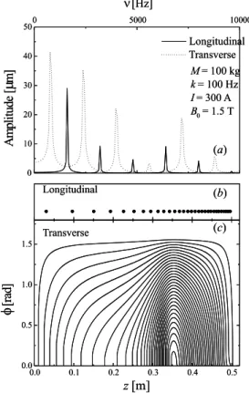
and c). These calculations were performed using Eqs. (7) and (14), and assumingl=1 m,c=C=1600 m/s,a=0.35 m, k=K=100 Hz, and using the parameters listed in Fig. 1c. For the transverse coil z=0.5 m, while for the longitudinal coil z = 0.45 m. Figs. 1b and 1c show one octant of the transverse, and half of the longitudinal coil layout. These unshielded gradient coils were designed by using the fast-simulated annealing method [18] to produce 32 and 44 mT/m, when driven by 300A currents, respectively. The amplitude of vibrations peaks at discrete frequencies, and does not exceed 50µm (Fig. 1c). It is obvious that longitudinal and transverse gradient coils produce different normal modes of vibration. Because the amplitude of sound in air is proportional to the amplitude of the coil vibrations [17], the linear increase of the gradient coil forces and vibrations withB0cause a logarithmic increase in SPL levels (in dB), in agreement with experimen-tal results [14]. In addition, Eq. (7) and (14) demonstrate that the amplitude of vibrations increases with coil radius and de-creases with coil mass. The relative amplitude of each normal mode depends on the current distribution.
FIG. 1: (a) Theoretical vibration amplitudes for harmonic driving currents as a function of frequency for longitudinal and transverse gradients. (b) Longitudinal coil layout. (c) Transverse coil layout (one octant). l=1m,a=0.35m,c=C=1600 m/s, andk=K= 100 Hz.
III. METHODS
To measure the mechanical vibrations of a gradient coil, three contact microphones were placed at different positions
on the inner surface of a whole-body shielded SONATA-Siemens gradient set. The mass, length and inner radius of this gradient assembly are 775kg, 1.245 m, and 0.3415 m, re-spectively. Three K2217 Siemens Cascade Gradient Power Amplifier (2000 V & 500 A) are used to produce gradient pulses with 44 mT/m peak amplitude and 0.25 ms rise-time. This gradient system was operated in a magnetic field ofB0= 4T and was driven by a Varian INOVA console.
The contact microphones (PZT) consisted of piezoelectric transducers (Radio Shack, 273-073A), which are ideal for use at high magnetic fields because they are non-magnetic. To estimate the frequency response of PZT microphones, we used a waveform generator to produce PZT-vibrations and power absorption of PZT microphones was measured as a function of frequency. These piezoelectric transducers have a non-uniform frequency response, being more sensitive to vibrations in the range of 500-3500 Hz. The microphones were glued on the inner wall of the gradient coil at posi-tions: (a,0,0),(0,a,0), and(0,−a,l/2)and were labeledx -PZT,y-PZT andz-PZT (a=0.3415 m). The output voltages of the microphones were digitized with a digital oscilloscope (LECROY 9354TM, 50ms trace, 500kHz-sampling rate, 16-bits dynamic range, high-impedance) and data analysis (FFT) was done in Microcal Origin (Microcal Software inc.) on a Personal Computer.
To measure the impulse response of the coil assembly, brief rectangular gradient pulses with 250A current amplitude (22 mT/m) and 500µsec-duration were applied, separately for each axis [19]. To evaluate the dynamic behavior of the gra-dient coil and identify potential higher-order normal modes of vibration, sine- and sinc-shaped gradient pulses were used. Sine pulses of 500 periods, with variable duration in the range 80-1000 ms, were used to sweep the frequency of the driving current in the range 500-5000 Hz. With these pulses, PZT sig-nals demonstrate an approximately 20ms-transient state, fol-lowed by a steady state, and another final 20ms-transient state (Fig. 5a). The amplitude of vibrations was measured in steady state conditions. Alternatively, sinc-pulses with 300 periods and 50ms duration were used to excite all high-order vibra-tion modes by a single waveform, by taking advantage of the flat, 6kHz-bandwidth spectral density of the sinc-pulses. In this case, signal acquisition was triggered at the maximum of the gradient pulse (Fig. 5b). The driving current was 30A for sine-, and 125A for sinc-gradient pulses
IV. RESULTS
Longitudinal impulse-response
Figure 2 shows damped oscillations of PZT-signals caused by a gradient pulse in the longitudinal gradient coil. The fric-tional resistance of the coil assembly, 2k=160 Hz, was ob-tained from Eq. (11) by fitting a mono-exponential decay to the envelope of the PZT signal. Thex- andy-PZT signals are smaller than thez-PZT signal due to the anti-symmetrical dis-tribution of magnetic force in the longitudinal gradient.
FIG. 2: Experimental vibration of coil assembly caused by a current-impulse in theGzcoil, as a function of time. Gradient amplitude 22
mT/m, pulse duration 0.5 ms. Dashed lines represent the exponential decay of damped oscillations.
FIG. 3: Fourier amplitudes of PZT signals from FIG.2.
in spectral density represent resonant vibration modes of the coil assembly. The exponential decay of signals in Fig.2 result in Lorentzian-shaped peaks of 40Hz full width half maximum (FWHM), in agreement with Eq. (11).
Thez-PZT spectral density has significant amplitude only in the range between 900-1400 Hz, and peaks at 1007, 1090,
and 1235 Hz (Fig. 3, bottom). These resonant modes, which correspond ton=2, have different resonance frequencies be-cause of the complex structure of the coil assembly. Higher vibration-modes were not observed in this experiment, prob-ably due to the limited bandwidth (∼2kHz) of the gradient pulses. Using Eq. (8) andl=1.25 m, the velocity of travel-ing waves for these resonant modes were calculated to bec= 1260, 1360, and, 1540 m/s.
Transverse impulse-response
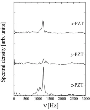
Figure 4 shows the spectral density of PZT signals follow-ing a brief gradient pulse on thex-gradient channel. While the resultingx-PZT spectrum shows resonance frequencies at 720 and 1220 Hz, they-PZT andz-PZT channels only exhibit the 720 Hz resonance. The even resonance mode (1220Hz) of the x-channel suggests that, due to imperfections of coil ends fix-ation, thex-transverse gradient can produce vibrations of the coil assembly’s surface aty=0 but not atx=0 in accord with a current distribution alongφin this gradient channel.
Our model suggests that the 720Hz resonance represents the fundamental mode (n=1) of axis-vibration due to coil bending. The velocity of traveling waves for these axis-vibrations was calculated to bec=1800 m/s, using Eqs. (8) and (15).
FIG. 4: Fourier amplitudes of coil vibration caused by a current-impulse in theGxcoil. Gradient amplitude 22 mT/m, pulse duration
0.5ms.
Dynamic-response experiment
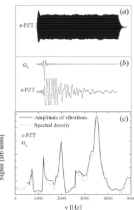
Figure 5c shows the spectral density of the x-PZT-signal when the Gx-coil is driven by sine-shaped (solid line) and sinc-shaped (dotted line) currents. Both methods show the same set of resonant modes.
FIG. 5: (a)x-PZT signal caused by a 500-period sine-shaped pulse in theGx-gradient coil. Gradient amplitude = 2.5 mT/m, pulse
du-ration = 400 ms (n= 1250Hz). (b)x-PZT signal caused by a 300-period sinc-shaped pulse in theGx-gradient coil. Maximum gradient
amplitude = 10 mT/m, pulse duration = 50 ms. (c) Amplitude of vi-brations in the assembly due to sine-gradient pulses (solid line) and sinc-gradient pulses (dashed line) in theGxcoil, as a function of
fre-quency.
FIG. 6: Frequency of resonant modes caused by sinc-shaped pulses in theGx-,Gy- andGz-gradient coils as a function ofn. Solid and
dashed lines are linear fits that represent Eqs. (8) and (15), fork<< ωn, andK<<Ωn.
Gz-spectrum peaks at different frequencies than Gx- andGy -spectra. This is due to the underlying difference in the current distributions and in the velocity of traveling waves forζ- and X-vibrations. Unfortunately, we were unable to make a com-parison between theory and experiment for the amplitudes of vibration, because for this particular gradient coil set the cur-rent distributions were unavailable to us. Such an analysis would be further complicated by the non-uniform frequency response of PZT microphones. Using the results of the im-pulse response experiment and Eqs. (8) and (15), high-order resonant modes were identified. Fig. 6 plots, for each gradient, the resonance frequency as a function ofn. Transverse gradi-ents produce odd normal modes of axis-vibration, while the longitudinal gradient produces even normal modes of surface-vibration, in agreement with the string model. Nevertheless, then=2 resonant mode of surface-vibration is also produced by transverse gradients, probably due to unbalanced fixations of coil ends. The slope of these data was used to determine the velocity of traveling waves to bec=1500 forζ-vibrations andC=1733 m/s forX-vibrations.
V. CONCLUSION
[1] S. A. Counter, A. Olofsson, H. F. Grahn, and E. Borg, J. Magn. Reson. Imaging7, 606 (1997).
[2] P. A. Bandettini, A. Jesmanowicz, J. Van Kylen, R. M. Birn, and J. S. Hyde, Magn. Reson. Med.39, 410 (1998).
[3] G. F. Eden, J. E. Joseph, H. E. Brown, C. P. Brown, and T. A. Zeffiro, Magn. Reson. Med.41, 13 (1999).
[4] Z-H Cho, S-C Chung, D-W Lim, E. K. Wong, Magn. Reson. Med.39, 331 (1998).
[5] M. R. Elliott, R. W. Bowtell, and P. G. Morris, Magn. Reson. Med.41, 1230 (1999).
[6] Y. Yang, A. Engelien, W. Engelien, S. Xu, E. Stern, and D. A. Silbersweig, Magn. Reson. Med43, 185 (2000).
[7] J. Hennig, and M. Hodapp, BURST imaging. MAGMA1, 39 (1993).
[8] F. Hennel, F. Girard, and T. Loenneker, Magn. Reson. Med.42, 6 (1999).
[9] F. Hennel J. Magn. Reson. Imaging13, 960 (2001).
[10] Z. H. Cho, S. T. Chung, J. Y. Chung, S. H. Park, J. S. Kim, C.
H. Moon, and I. K. Hong, Magn. Reson. Med.39, 317 (1998). [11] P. Mansfield, B. L. W. Chapman, R. Bowtell, P. Glover, R. Coxon, and P. R. Harvey, Magn. Reson. Med.33, 276 (1995). [12] P. Mansfield, and B. Haywood MAGMA8(Suppl), 55 (1999). [13] P. Mansfield, B. Haywood, and R. Coxon, Magn. Reson. Med.
46, 807 (2001).
[14] D. L. Price, J. P. De Wilde, A. M. Papadaki, J. S. Curran, and R. I. Kitney J. Magn. Reson. Imaging13, 288 (2001). [15] Y. Wu, B. A. Chronik, C. Bowen, C. K. Mechefske, and B. K.
Rutt, Magn. Reson. Med.44, 532 (2000).
[16] R. A. Hedeen, and W. A. Edelstein, Magn. Reson. Med.37, 7 (1997).
[17] P. Mansfield, P. M. Glover, J. Beaumont, Magn. Reson. Med. 39, 539 (1998).
[18] D. Tomasi, Magn. Reson. Med.45, 505 (2001).