Brazilian Journal of Physics, vol. 36, no. 1A, March, 2006 1
Study of Turbulent Flow using Half-Fourier Echo-Planar Imaging
A. O. Rodr´ıguez
Centro de Investigaci´on en Imagenologia e Instrumentaci´on M´edica, Universidad Aut´onoma Metropolitana Iztapalapa, Av. San Rafael Atlixco 186, M´exico, D. F., 09340. M´exico
Received on 16 May, 2005; accepted on 28 November, 2005
The Echo-Planar Imaging technique combined with a partial Fourier acquisition method was used to ob-tain velocity images for liquid flows in a circular cross-section pipe at Reynolds number of up to 8000. This partial-Fourier imaging scheme is able to generate shorter echo times than the full-Fourier Echo-Planar Imaging methods, reducing the signal attenuation due to T2* and flow. Velocity images along the z axis were acquired with a time-scale of 80 ms thus obtaining a real-time description of flow in both the laminar and turbulent regimes. Velocity values and velocity fluctuations were computed with the flow image data. A comparison plot of NMR velocity and bulk velocity and a plot of velocity fluctuations were calculated to investigate the feasi-bility of this imaging technique. Flow encoded Echo-Planar Imaging together with a reduced data acquisition method can provide us with a real-time technique to capture instantaneous images of the flow field for both laminar and turbulent regimes.
Keywords: Turbulent flow; Imaging; Echo-planar imaging
I. INTRODUCTION
In order to distinguish transient phenomena with NMR imaging, the use of ultra-fast flow imaging techniques is re-quired. Under these circumstances it is essential to have an observation time short relative to the time scale of the phys-ical property to be measured. Transient phenomena include, for example, turbulent flow at high Reynolds number, flow and dispersion through porous media, and extensional defor-mation. It has been proved that Echo-Planar Imaging can suc-cessfully quantified spatial and temporal characteristics of tur-bulent flow in pipes [1-5]. Other flow MRI techniques have been proposed by other groups [6-8].
In this paper, a variant of the Echo-Planar Imaging (EPI) technique [1] is used to determine flow for the laminar and tur-bulent regimes. This version includes a partial Fourier tech-nique [9] which is able to generate shorter echo times than the full-Fourier methods such Modulos Blipped Echo-Planar Imaging Single Shot (MBEST) [10], reducing the signal at-tenuation due to T2* and flow. The real-time flow measure-ment method proposed by Guilfoyle and et al. [1] was used to measure the velocity in the laminar regime and turbulent reg-imen. This mathematical expression was also used to derive a formula for the turbulent case. Then, a combination of the method above and a scheme introduced by Gatenby and Gore was used to measure the velocity fluctuations of the turbulent regime [1].
Gatenby and Gore have developed a phase-dependent ex-pression to measure the turbulence intensity as a function of the gradient waveform and velocity fluctuation. We used the theoretical model of [1] for the long-lived regime together with a modified version of the flow EPl technique, and called Half Fourier Echo-Planar Imaging (HF EPI) [9], to measure turbulence intensity in pipe flows. Flow images for both regimes were acquired and their corresponding velocity val-ues were also computed to investigate the feasibility of this MRI technique. In this paper, we present the results of stud-ies of laminar and turbulent flow using Half-Fourier EPI. Our
specific aim was to investigate whether our flow imaging tech-nique was able to measure both quantitative and qualitative in-formation in real time for the laminar flow and turbulent flow.
II. METHOD
A flow-encoding gradient is used prior to the EPI experi-ment incorporating a 1800pulse to overcome magnetic field inhomogeneities. The flow-encoding sequence 900-τ-1800− 900x or yor y pulse train prior to the standard EPI sequence. This is depicted in Fig. 1. Each gradient is applied for a time t. After the second flow encoding gradient pulse, the spin mag-netisation is tipped back along the main field axis with a 900 pulse. A spin phase scrambling gradient is then applied to destroy any remaining signal before applying a normal EPI experiment to image the residual longitudinal magnetisation created by the preceding 900pulse of the flow-encoding se-quence. Two components of the magnetisation are consid-ered; the first from the static spinsMstat(=Mx=M0cos(β)) and other from the spinsMV(=My=M0sin(β)), flowing with constant velocityV, which undergone a phase shiftβ given by [1]:
β=γGVNMR(τ2+τtr) (1)
whereγis gyromagnetic ratio,tandGare the duration time and strength of the gradient,τis the delay time. The phase variation is directly proportional to the spin velocity.
2 A. O. Rodr´ıguez
FIG. 1: Timing diagram for the RF pulses and flow-encoding gradi-ents.
echoes were used to generate a coarse map, which was used subsequently in phase correction [9]. Images for each com-ponent were acquired for diferentes flow rates whit the fol-lowing acquisition parameters: t= 12 ms andG= 4 mT/cm, tr=400µs(rise time), andτ= 2 ms in Fig. 1. Each experiment was repeated for flow rates from 0 to 1770 ml/cm (0-30 cm/s). This range allows both laminar flow and turbulent flow to be developed. All experiments were performed on the Notting-ham 0.5T imager.
The flow encoding sequence which proceeded the HF EPI read-out module is shown in Fig. 1. The magnitude of the signal is:
SA=S0sin(β) (2a)
SB=S0cos(β) (2b)
depending upon whether the 2nd RF pulse is applied along the X(cosine) orY(sine) axis in the rotating frame [1,9].βis the phase shift of the spins flowing along the pipe. We computed the velocity for the two regions, laminar and turbulent using two different expressions. To measure the flow in the laminar region the following velocity expression was derived from Eq. (1):
VNMR=
arctan(SA/SB) γG(τ2+τt
r)
(3)
From the signal expression from [11] for the case of long-lived fluctuations compared to both t and τ, and the flow-sensitive gradient diagram in Fig. 1, the velocity fluctuation is:
u2®
= arctan(SA/SB)
γ2G2(t2+τ(t+t
r) +3ttr+2tr2)2
(4)
wheretr is the rise time, the variableβ can be the velocity
VNMR(laminar flow) of Eq. (1) or the velocity fluctuationu2® (turbulent flow) of Eq. (4).
III. RESULTS AND DISCUSSION
Half-Fourier EP images were acquire of a circular cross section for the static case, laminar and turbulent regime. Flow
FIG. 2: Phantom images of stationary water: sine (weak) and cosine (strong) components.
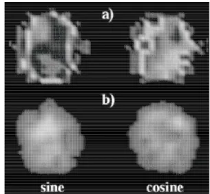
FIG. 3: Phantom images of components sine and cosine for: a) lam-inar regime and b) turbulent regime.
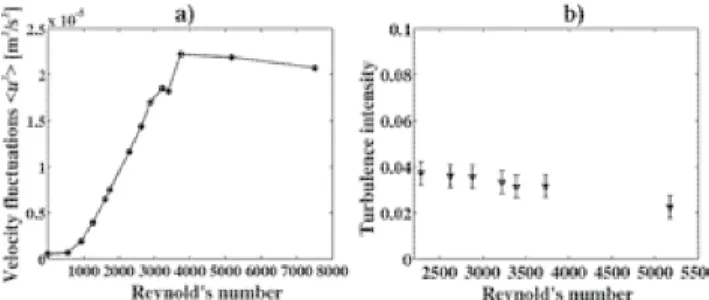
images for each flow rate were obtained and their correspond-ing velocities were computed with the pipe geometry and the flow rate. Fig. 2 shows two cross-sectional images of the water phantom (right lower corner) and pipe for the static case. Sine and cosine components for the laminar and turbulence cases were also computed and shown in Fig. 3. From the images showing laminar behaviour a velocity profile was plotted and shown in Fig. 4. Fig. 5 shows a graph of the NMR velocity calculated from the flow images and Eq. (3) against the Bulk velocity computed as mentioned above. The linear regression of the experimental data stresses the excellent agreement of the NMR velocity the actual bulk velocity in the pipe. Thus, it can be implied that NMR velocity = Bulk velocity. This indi-cates a linear function over the laminar range as expected for the laminar behaviour. Fig. 6a) shows that the experimentally-acquired values of u2® plotted against Reynold’s number. There is no need to use a general fit to calculate the veloc-ity fluctuations for the long-lived regime as reported in [11].
Gatenby and Gore reported a constant value of u2®
in-Brazilian Journal of Physics, vol. 36, no. 1A, March, 2006 3
FIG. 4: Velocity profile of laminar flow obtained in transverse section across the circular pipe.
FIG. 5: Correlation between the average velocity NMR velocity mea-sured using Half- Fourier Echo-Planar Imaging with the value of the bulk velocity determined from the known flow rate and the geometry of the tube.
crement can be observed as a function of the flow rate in this region. It is very unlikely that running water from a tap can reach a complete laminar regimen since may factors affect the behaviour of the water flow. These velocity fluctuations do not drastically affect the velocity measurements as shown in [11], however these small fluctuations can be measured with HF EPI. For Re>2500 velocity fluctuation values grow rapidly with flow rate.
Our data is in good agreement with this well-known and es-tablished threshold of turbulence. It then seems that our flow MRI technique is able to detect velocity fluctuations which are
FIG. 6: a) Experimental velocity fluctuation ( u2®
) plotted against Reynolds number for pipe flow. a) Experimental turbulent intensity (TI =
u2®1/2
/U plotted against Reynold’s number: Uis the flow velocity.
not necessary caused by the turbulent behaviour of the flow. This is probably due to the better temporal resolution of HF EPI. Fig. 6b) plots the turbulent intensity, for the flow rates at which turbulent flows has been established (Re>2500). The turbulent intensity is approximately constant which is in good agreement with data reported in [11]. The method proposed here allows to directly obtain experimental measurements of the velocity fluctuations via a phase map formed with the two images determined with the flow encoding sequence and Eqs. (2) and (3). Despite the lower spatial resolution of a low field scanner, our data shows good agreement with the values re-ported in the literature.
It has been proved that flow encoded EPI together with a re-duced data acquisition method can provide us with a real-time technique to measure laminar behaviour and velocity fluctu-ations for flow in pipes for Reynolds up to 80000. Guilfoyle and coworkers’ approach can be easily modified to derive an expression to directly measure turbulent intensity and velocity fluctuations. In simple pipe flow, the onset of turbulence can then be accurately detected without disturbing the flow. This scheme reveals the potential to obtain relevant flow informa-tion for both laminar and turbulent behaviour of pipe flow.
Acknowledgements
I wish to express my gratitude to Sir Peter Mansfield for his supervision and advise during this work.
[1] D. N. Guilfoyle, P. Gibbs, R. J. Ordidge, and P. Mansfield, Magn. Reson. Med.18, 1 (1991).
[2] K. Kose, J. Magn. Reson.92, 631 (1991).
[3] J. C. Gatenby, J. C. Gore, J. Magn. Reson.121, 193 (1996). [4] A. J. Sederman, M. D. Mantle, C. Buckley, and L. F. Gladden,
J. Magn. Reson.166, 182 (2004).
[5] S. I. Han, P. T. Callaghan, J. Magn. Reson.148, 349 (2001). [6] Y. Q. Song, Ulrich M. Scheven, J. Magn. Reson.172, 31 (2005). [7] K. Kose, J. Phys. D: Appl. Phys.23, 981 (1990).
[8] A. J. Sederman, M. D. Mantle, and L. F. Gladden, J. Magn. Reson.161, 15 (2003).
[9] A. Rodriguez, B. Issa, R. Bowtell, and P. Mansfield, IV, Supp.
254, 100 (1996).
[10] A. M. Howseman, M. K. Stehling, B. Chapman, R. Coxon, R. Turner, R. J. Ordidge, M. G. Cawley, P. Glover, P. Mansfield, and R. E. Coupland, Br. J. Radiol.61, 822 (1988).