MRI Relaxometry: Methods and Applications
A. A. O. Carneiro, G. R. Vilela, D. B. de Araujo, and O. Baffa
Departamento de F´ısica e Matem´atica, FFCLRP, Universidade de S˜ao Paulo, 14040-901, Ribeir˜ao Preto – SP, Brazil
Received on 21 October, 2005
Aspects of magnetic resonance relaxation measurements in human tissues are discussed. The influence of pulse sequences and parameters are compared and analyzed for different tissues. By controlling the acquisition parameters and data fitting the relaxation rate can be useful in several clinical situations. The influence of repetition and echo time, predicted in sequences of signal acquisition, on measurement of transversal relaxation time (T2) was evaluate using simulated MRI signal.
Keywords: Magnetic resonance imaging; MRI
I. INTRODUCTION
The use of magnetic resonance imaging (MRI) as a quanti-tative tool has attracted great interest by various research cen-ters. The improvement in the sensitivity and the reduction of the subjectivity of visual evaluation created a significant im-pact on diagnosis of tissue abnormalities, such as tissue iron overload.
The most common MRI techniques for quantitative diag-nosis at the lesion level are relaxometry (R), magnetization transfer (MT) and Spectroscopy (MRS). However, one impor-tant issue is standardizing a calibrating protocol to be used in different scanners that is imperative to allow the use of MRI as a quantitative tool.
Most commonly, MRI can be weighted in T2 (transver-sal relaxation time) and/or T1 (longitudinal relaxation time), where the nature of the image contrast is based on relative con-tributions from different tissues. On the other hand, one can create a map, based on the relaxation time itself, also known as relaxometry. Such map can be constructed considering each one of these parameters separately or together. Generally, ap-plications for tissue characterization make use of spin-echo sequences, with two or more different times of echo (TE) and a long time of repetition (TR), and are currently being applied to evaluate brain, breast, muscle and liver tissue [1-7].
We present here the relevant principles of T2 weighted re-laxometry. Section 2 reviews important aspects of relaxation rate (R2) for specific tissues and specific MRI sequences ded-icated to relaxometry. With these sequences an R2 map can be produced and overlaid onto the images. Section 2.1 discusses the condition under which the TE for each tissue optimizes the sensitivity of the exam. In section 2.2 we present image ac-quisition and processing that allows the best fit between signal intensity and TE. Details and results of particular applications to evaluate tissue lesions and liver iron overload by relaxom-etry are discussed on section 3. The variance between the experimental data and fitted curve will also be discussed.
II. THEORY AND METHODS
The theory of relaxometry, or the measurement of ation rates, is based on the physical aspects of nuclei
relax-ation to the ground state after being excited by an RF pulse. This relaxation is produced by randomly occurring variations in the local magnetic field strength. T2 relaxation is due to a dephasing of individual magnetic moments of the protons, and begins immediately after the RF pulse. Protons will become out of phase as they experience a slightly different magnetic field and then rotate at a slightly different frequency. This transversal relaxation occurs both due to magnetic field inho-mogeneities produced by the magnet or by magnetic particles present in the tissues and due to movement of the molecules in the tissue.
A. Imaging acquisition and processing
Relaxometry maps may be generated either by spin-echo or by gradient echo sequences. In the latter, T2∗ is being measured, rather than T2. Therefore, the results may be nois-ier since the influence of inhomogeneities in the magnetizing field is greater.
To generate a map of relaxation rate (R2=1/T2) or relax-ation time (T1 or T2), using spin echo sequences, at least two images are necessary. The sensitivity of this technique de-pends on sequence, time of repetition (TR), time of echo (TE), the number of images acquired with different TE, and on the model adopted for fitting the experimental data.
showed that a single spin echo sequence may be used to im-prove the precision of the relaxometry technique to evaluate iron overload in tissue [9].
Increasing TR also increases the signal-to-noise ratio (SNR) in relaxometry evaluation. Generally, TR is at least three times T1. However, increasing TR increases the acqui-sition time. Another important aspect in relaxometry is the value and the number of TEs. The larger the number of TEs the better is the SNR ...[9]. The values of TE should be cho-sen in a range centered close to the values of T2 for the sam-ple. A value of T2 close to TE, but sufficiently longer than T2 fluctuations in region of interest (ROI) of the tissue, will give more accurate T2 measurements.
For tissues where the signal intensity decays rapidly, such as tissues with iron overload, the signal intensity (SI)versus TE is well fit by a single-exponential function [7,10]. More-over, SNR increases when the images are pre-processed by a smooth filter. However, this process decreases the spatial res-olution of the relaxometry map [11]. It is common to quantify T2 values by the regression of the natural logarithm of the sig-nal intensity versus TE with two exponential functions. The T2 determination is uncertain if the relaxation of the SI does not follow a single-exponential behavior. An even more seri-ous uncertainty in T2 results appears if an offset signal is not subtracted from the SI before the curve fitting. In practice, a single exponential decay of the signal intensity (SI)versusTE should not be applied for all tissues as it will be show in the next section.
In quantitative magnetic resonance imaging, the accuracy of an image derived from relaxation rates is primarily depen-dent on the processing of the image data that must be un-corrupted by acquisition artifacts [12]. Respiratory motion, for example, is a predominant source of artifacts, especially for axial MR images of the abdomen [13]. Besides tradi-tional noise suppression, another important method of image processing is providing a reference signal intensity to com-pensate differences of image brightness from the same tissue acquired with different TE. One can use a homogeneous phan-tom with an MRI signal intensity equivalent to the average signal of the tissue being investigated. Therefore, the value of the intensity from the phantom for each TE may be used to correct the scanner drift of the signal intensities from the tissue being investigated [6].
B. T2 analysis by simulated data
To the first approximation, the relaxation of signal intensity, following a spin-echo pulse sequence assumes an exponential decay, given by the expression [14]:
SSE =So
·
1−2e−
T R−T E/2 T1 +e−T ET1
¸
e−T ET2, (1)
where S0 is the proton density, T1 and T2 are longitudinal
and transversal relaxations, respectively. The parameters (So,
T1 and T2) characterize the tissue properties and the image
contrast should be weighted with each one of these parameters by controlling TE and TR during the image acquisition.
In practice, the use of equation 1 to fit the SSE versusTE
curve poses a difficult task. Equation 1 does not separate T1 and T2 contributions sufficiently to detect fine abnormalities of tissues. Generally, one can eliminate T1 contribution from expression 1 by using a TR much longer than T1, as most biological tissues have a T1 shorter than 250 ms. When the tissue has a long T1, as in the Cerebral Spinal Fluid (CSF) (T1∼2500 ms and T2∼1400 ms), a very long TR will be nec-essary in order for T2 to dominate the signal decay.
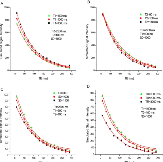
The dependency of the MRI signal on TE was simulated using equation 1 for different values of T1, T2 and TR. As shown in Fig. 1, the signals were plotted using. The fol-low procedure: a) large variation on T1 (500, 1000, 1500), T2=100 ms; TR=2500 and S0= 1000; b) 10% of variation
on T2 (90, 100, 110), T1 = 500 ms, TR=5xT1 and S0=
1000; c) 10% of variation on S0 (900, 1000, 1100), T2=
100 ms, T1=500, TR=5xT1 ms; d) large variation on TR (1000,2000,3000), T2=100 ms, T1=1000 ms and S0= 1000).
A Gaussian noise of 1% was added to all simulated signals to represent statistical fluctuations of detection system and the random variations of the local electromagnetic field due to eddy currents induced within tissues.
The simulated signals were fitted using single and bi-exponential curve, according to:
SSE=Soe
−T ET
2 +Soffset , (single−) (2)
SSE =So1e
−T E T21+S
o2e
−T E T22 +S
offset , (bi−) (3)
where Sois the maximum signal from the sample and Soffset
is an offset signal from the system.
To evaluate the variation on parameters S0 and T2, the fit
was made considering two methods: all arbitrary parameters free and some parameters fixed. This second one was made using the following protocol:
Single-exponential: offset was considered fixed and equal to zero;
Bi-exponential: S01 equal to S02 and the offset was fixed
equal to the noise level estimated for each signal. In the sim-ulated data the offset was zero.
Simulations were performed using a program written in MatLab 6.5 and the relaxometry parameters were estimated by fitting the simulated data using a non-linear curve fit ac-cording toχ2minimization algorithm, based on Levenberg-Marquardt method, with an interval of confidence of 95%.
0 50 100 150 200 250 300 0
200 400 600 800 1000 A
TR=2500 ms T2=100 ms S0=1000
S
im
u
la
te
d Sign
al I
n
te
ns
it
y
TE (ms)
T1= 500 ms T1=1000 ms T1=1500 ms
0 50 100 150 200 250 300
0 200 400 600 800 1000 B
TR=2500 ms T1=500 ms S0=1000
S
im
u
la
te
d
S
ig
n
a
l In
te
n
s
it
y
TE (ms)
T2=90 ms T2=100 ms T2=110 ms
0 50 100 150 200 250 300
0 100 200 300 400 500 600 700 800 900 1000 C
TR=2500 ms T1=500 ms T2=100 ms
Sim
u
la
ted Signal I
n
tens
it
y
TE (ms)
S0=900 S0=1000 S0=1100
0 50 100 150 200 250 300
0 100 200 300 400 500 600 700 800 900
D
T1=1000 ms T2=100 ms S0=1000
Si
mul
a
ted Si
gnal
Intens
it
y
TE (ms)
TR=1000 ms TR=2000 ms TR=3000 ms
FIG. 1: Signal intensity versus TE values simulated from equation 1 and fitted by equation 2. a) large variation on T1, with TR>>T1; b)10% of variation on T1 for TR=2.5*T1; c) 10% of variation on T2, with TR=2,500 ms, T1= 500 ms; d) TR=[T1, 2T1and 3T1] , with T1=1,000 ms, T2=100 ms.
equivalent to T1, small variations will result in a considerable modification on signal amplitude.
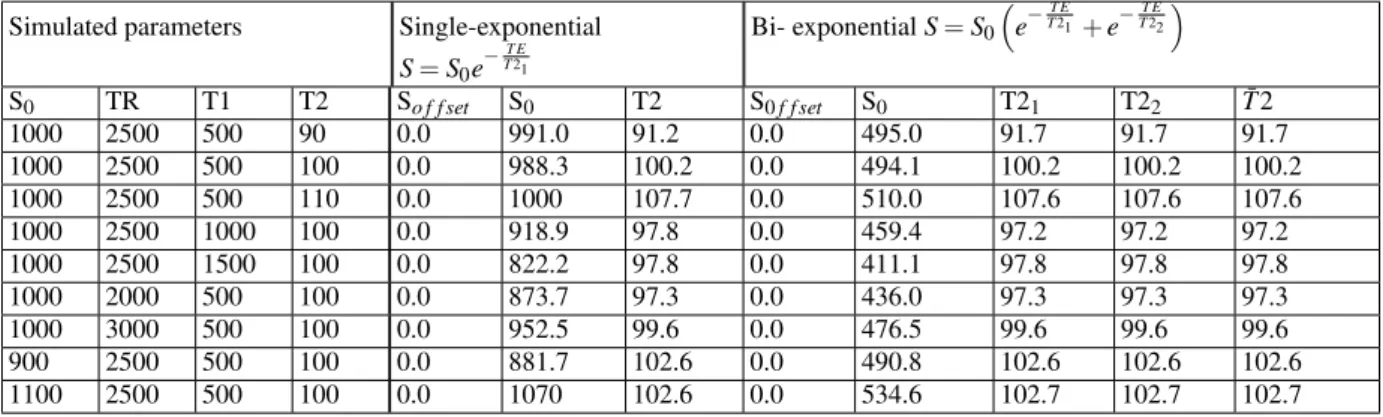
Table 1 and 2 show the distribution of relaxometry parame-ters obtained from single- and bi-exponential fit of the simu-lated curves of Fig. 1. Although the offset level (Soffset)has
been considered zero in the simulated data, a fluctuation of about 1%, relative to proton density (S0)was observed. The
shorter TR, the larger is the deviation of T2 obtained both by single- and by bi-exponential fit.
The absolute deviation of T2 for all conditions of simula-tion presented in table 1 and 2 was smaller when T2 was ob-tained considering the offset fixed and equal zero and with equal amplitudes of S01and S02for the bi-exponential curve.
For these parameters, the value obtained for T2 was similar for both single and bi-exponential fits.
When all parameters of equation 3 were allowed to be ad-justed, the fluctuation in both T21and T22was large. Fig. 3
shows that using a bi-exponential fit (equation 3), results in large uncertainties in T2 values. Besides, the number of it-erations necessary to have the fitted data converging to a 95% confidence is greater than when some parameter is maintained
fixed.
TABLE I: Relaxometry parameter obtained from Single- and Bi-exponential fitting of simulated MRI signal from a spin-echo sequence versus TE. In this table ¯T2 is the average value of T2. Shadowed cells show the varying parameters.
Simulated parameters Single-exponential
S=S0e−
T E
T2+So f f set
Bi-exponential
S=S01e
−T E T21 +S02e−
T E
T22 +So f f set
S0 TR T1 T2 So f f set A T2 So f f set S01 S02 T2,1 T2,2 T¯2
1000 2500 500 90 7.2 988.5 89.1 7.2 491.2 497.3 89.0 89.0 89.0
1000 2500 500 100 13.4 982.7 96.1 2.5 486.0 495.0 96.9 103.9 100.4
1000 2500 500 110 -5.0 1003 109.3 2.9 496.0 499.0 99.9 114.0 107.0
1000 2500 1000 100 11.4 914.3 94.2 6.1 444.3 468.0 102.8 90.7 96.8
1000 2500 1500 100 -4.1 824.0 99.3 7.2 385.8 428.8 101.5 91.4 96.5
1000 2000 500 100 -12.0 878.9 101.7 15.9 417.2 449.5 95.2 90.6 92.9
1000 3000 500 100 -10.0 957.2 102.7 15.2 435.8 501.0 98.8 94.5 96.7
900 2500 500 100 4.2 879.8 101.1 6.9 403.0 477.9 105.6 95.3 100.5
1100 2500 500 100 4.8 1067 101.4 8.4 489.7 578.8 105.6 95.5 100.6
TABLE II: Relaxometry parameter obtained from Single- and Bi-exponential fitting of simulated MRI signal from a spin-echo sequence versus TE. In this fit, the offset was maintained fixed. Shadowed cells show the varying parameter.
Simulated parameters Single-exponential
S=S0e
−T E T21
Bi- exponentialS=S0
³
e−TT E21+e−TT E22´
S0 TR T1 T2 So f f set S0 T2 S0f f set S0 T21 T22 T¯2
1000 2500 500 90 0.0 991.0 91.2 0.0 495.0 91.7 91.7 91.7
1000 2500 500 100 0.0 988.3 100.2 0.0 494.1 100.2 100.2 100.2
1000 2500 500 110 0.0 1000 107.7 0.0 510.0 107.6 107.6 107.6
1000 2500 1000 100 0.0 918.9 97.8 0.0 459.4 97.2 97.2 97.2
1000 2500 1500 100 0.0 822.2 97.8 0.0 411.1 97.8 97.8 97.8
1000 2000 500 100 0.0 873.7 97.3 0.0 436.0 97.3 97.3 97.3
1000 3000 500 100 0.0 952.5 99.6 0.0 476.5 99.6 99.6 99.6
900 2500 500 100 0.0 881.7 102.6 0.0 490.8 102.6 102.6 102.6
1100 2500 500 100 0.0 1070 102.6 0.0 534.6 102.7 102.7 102.7
III. SINGLE- VERSUS BI-EXPONENTIAL FIT
Generally, T2 has been evaluated using single- or bi-exponential fitting to the experimental data with no attention given to the mathematical protocol to best adjust appropriate parameters. For example, the value of T2 obtained from an exponential fit could be strongly influenced by the choice of the amplitude of the signal offset (So f f set). A bi-exponential
function makes the fitting more critical, since besides the vari-ation of amplitude of offset, the exponential terms will interact to permit the best fit. In this case, both the amplitude and re-laxation time parameters fluctuate between mean values. This criticality is clearly observed from simulated results presented in section 2.1. For example, for 5 simulated signals with 1% of noise, generated using the same parameters (TR=2,500 ms, T1=500ms, and T2=100ms) the fluctuation of the adjusted pa-rameter was about 0.8 % when the single-exponential fitting was done keeping the offset fixed and about 4% when all other parameters were free. The results in table 1 and 2 show the criticality of the bi-exponential fit when all 5 parameters were free to be adjusted. The adjusted parameters were more stable when both amplitudes were considered equal and the offset was fixed. This mathematical procedure of getting the relax-ometry parameters guarantees the best resolution of this pro-cedure to detect small relaxation changes of tissues.
IV. IN VIVOAPPLICATIONS
In this section we will present examples of relaxometry applications to quantify T2 or R2 values in some biological tissues. To guarantee a relative comparison between differ-ent tissues, the same sequence and processing were used to generate R2 maps. Images were acquired in a 1.5 T scanner (Siemens Magneton Vision) using a multi-spin-echo sequence (16 echoes) with TE multiples of 22.5 ms [22.5, 45,. . . 360 ms], with long TR (TR¿= 2,000 ms). Due to the long repeti-tion time, no respiratory-gating or breath-holding techniques were employed to avoid movement artifacts. R2 maps were superposed onto an intensity image for best visualization.
A. Tissue Iron Overload
The higher the concentration of iron stored on the tissue, the shorter will be the value of T2 (longer R2), and the shorter should be the TE values. Generally, patients that regularly re-ceive blood transfusions have the level of iron in the body in-creased, especially those who are not submitted to iron chela-tion therapy. The organs that most accumulate iron are liver, heart and spleen.
0 20 40 60 80 100 120 140 160 180 200 220 0
50 100 150 200 250 300 350 400 450 500
A
Me
a
n
In
te
n
s
it
y
TE (ms)
Single-Exponencial Fit Spleen (T2 = 75.3 ms) Liver (T2 = 63.9 ms)
0 20 40 60 80 100 120 140 160 180 200 220 2.5
3.0 3.5 4.0 4.5 5.0 5.5 6.0 6.5
B
ln
(M
ean I
n
te
n
s
it
y
)
TE (ms)
Spleen (75.3 ms) liver (63.9)
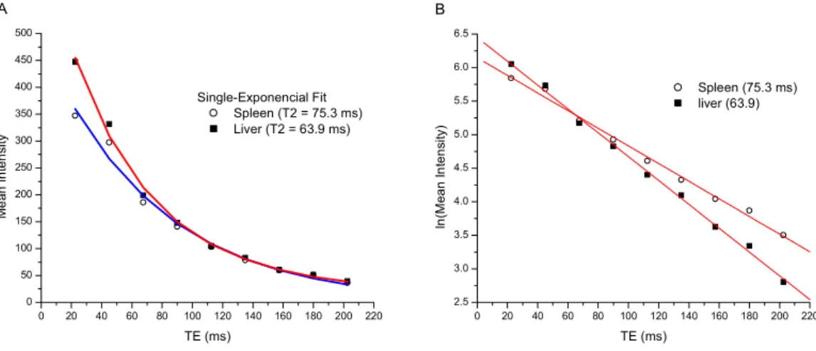
FIG. 3: Single-exponential fit of mean intensity signal versus TE for liver and spleen region drawn on Fig. 2 shown in a linear (A) and logarithmic (B) scale.
FIG. 4: Map of relaxation rate R2 (1/T2) of the left breast superposed on T2-weighted image. This image was acquired on a 54 year old woman.
controls, on the protocol of measurement and on processing [9].
Figure 2 shows an R2 map, acquired in an asymptomatic subject (40 year old), from the liver and spleen region. The R2 was obtained by fitting the signal intensity in a pixel-by-pixel basis using a single-exponential curve. A 3x3 matrix mask smooth filter was applied to reduce respiratory artifacts. As liver and spleen tissues have a short T2 (∼40 ms), only the 9 first images, with TE multiples of 22.5 ms, were used. Fig. 3 shows the fit of the mean intensity versus TE, for both liver and spleen regions marked on Fig. 2. As T1 for these tissues are shorter than the TR, a single-exponential curve gives a good fit.
0 20 40 60 80 100 120 140 160 180 200 220 0
100 200 300 400 500 600 700 800 900 1000 1100 1200 1300 1400 1500 1600 1700
Mean I
n
tensi
ty
TE (ms)
Fibrogandular (T2 = 75 ms) Lesion (T2 = 356 ms) Adipose (T2 = 52 ms)
FIG. 5: Single-exponential fit of mean intensity signalversus TE from three different region of the breast: fibrogandular tissue (∆); damaged tissue (o)and adipose tissue (♦)of the whole left breast area.
B. Breast relaxometry
Nowadays, there has been a marked increase in the use of MRI for breast tissue evaluation. Multiple research studies have confirmed the potential of relaxometry for early breast cancer detection, diagnosis, and evaluation of response to therapy [16]. From T2-weighted images, differentiation be-tween adipose and glandular tissue types is clear due to their distinctly different T2 values. For the same reason relaxome-try differentiate easily normal from abnormal tissue.
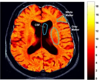
FIG. 6: Map of relaxation rate R2 of an axial slice from a human brain superposed on T2-weighted image. Regions with short T2 are indicated with bright color and long T2 with black color.
0 20 40 60 80 100 120 140 160 180 200 220 0
100 200 300 400 500 600
M
ean Intensi
ty
TE (ms)
White Matter (T2 = 97 ms) Gray Matter ( T2 = 93 ms) CSF (T2 = 1530 ms)
FIG. 7: Single-exponential fit of mean intensity signal versus TE from different brain tissues of an axial slice.
C. Brain Relaxometry
T2 relaxometry in human brain has also been successfully used to differentiate normal from abnormal tissues. Increased signal on T2-weighted MRI is a feature to identify cerebral abnormalities. The measurement of T2 has been shown to be useful in the assessment of hippocampal sclerosis, particularly if there are only subtle changes that may not be evident visu-ally, in the evaluation of some tissue regions as contralateral hippocampus, amygdale, white matter, and thalamus [1,2,17]. Figure 6 shows an R2 map of an axial slice from a 48 year old woman brain, superimposed onto a T2 weighted image. This map was generated by fitting single-exponentials of cor-responding pixels of images obtained using the same multi-spin sequence and protocol of processing presented in the pre-vious sections.
Due to the large number of subdivisions of brain anatomy, sometimes it is difficult to select a small region to perform re-laxometry. Nevertheless, with a whole brain map, small seg-mented regions are selected and the mean T2 value, or his-togram, for each segment can be generated. Fig. 7 shows the single-exponential fit for the three regions selected on Fig. 6. The T2 values in white and gray matter were 97 and 93 ms, respectively. For the CSF T2 was 1,530 ms.
Table 3 shows the relaxometry parameters for liver, spleen, breast and brain tissues, determined using the same procedure used for the simulated study. The signal of offset was esti-mated getting the signal intensity when the TE was infinite. A fitting was also made for zero offset.
V. DISCUSSION
In this study, we observed that when the T2 is being deter-mined by a single-exponential fit, the offset should be mea-sured and maintained fixed when evaluating variation on re-laxometry measurement caused by abnormalities on a specific region. When using a linear fit to the natural logarithm of the signal intensity without first subtracting an offset amplitude, the T2 of the tissue will be uncertain and the data will not be well fit. The relaxometry parameter will be unable to evalu-ate small abnormalities in tissue. For example, when only two echoes are used for a relaxometry measurement, it is impos-sible to predict an offset signal and the T2 value is obtained by linear fitting of the natural logarithm of the signal intensity versus TE.
In fibroglandular and adipose breast tissues the relaxation times (T21and T22)obtained from a bi-exponential fit were
different. It implies that although the data were visually well fitted by a single-exponential function, the relaxation of signal has different rate in different portions of the curve. So, fitting the data using a bi-exponential function with the amplitude of both exponential terms equal (S01=S02)and one offset value
fixed for the same study, we are looking at the relaxometry rate of segments that are proton density and T2 – weighted separately. If the image was acquired using the ideal range for TE adjusted on sequence, the amplitude obtained from this last protocol of fitting should be approximately equal to the amplitude of signal for TE equal to T2 of the tissue.
The R2 map has a contrast equivalent to a T2 weighted image with the advantage of representing quantitative infor-mation that is extremely useful for abnormality diagnosis. In summary care must be taken to standardize the whole proce-dure for proton relaxation measurements in MRI in order to give clinical value to this parameter.
TABLE III: Relaxometry parameter obtained from Single- and Bi-exponential fitting of MRI signal from a spin-echo sequence versus TE on liver, spleen, breast and brain region. The superscript “F” means fixed parameter during the fitting.
Tissue Single-Exponential Bi-Exponential
y0 So T2 y0 So1 T21 So2 T22
Liver 23.7 648.4 55 24.8 307.2 54.2 342.7 55.1
0F 636.5 63.0 23F 323.9 55.3 323.9 55.3
Spleen 2.8 484.5 73.9 2.8 242.8 73.9 243.8 73.9
0F 484.5 75.3 2.8F 242.1 73.9 242.1 73.9
Breast: Fibroglandular 23.3 1012.7 65.9 23.3 705.6 65.9 307.0 70.0
0F 993.7 73.5 23.3F 512.2 64.8 512.2 72.0
Breast: Adipose 165.3 1931.0 75 165.3 964.0 75.0 967.6 75.0
0F 1970 96.7 165.3F 965.8 75.0 965.8 75.0
Breast: Lesion 38.7 1241.9 146.3 38.7 1160.0 190 273.7 32.0
0F 1333.7 206.3 38F 709.0 105.3 709.0 37.0
Brain: CSF 40 514.6 1638 42.6 256.0 1629 256 1629
0F 568.3 1767 40F 257.0 1631.0 257.0F 1631
Brain: Gray Mater 18.6 745.1 90.9 18.0 522.4 90.9 222.7 90.9
0F 741.1 100.2 18F 372.5 91.2 372.5F 91.2
Brain: White Matter 13.4 749.6 89.6 13.4 524.8 89.6 224.8 89.6
0F 746.5 96.1 13F 347.7 89.8 347.7 89.8
than TE. Because of the dispersion on MR signal, due to the intrinsic noise of MRI technique, the fitting of the data is criti-cal and a special attention is also necessary during mathemat-ical processing.
Acknowledgments
The authors are grateful to Prof. D. T. Covas, M. A. Zago, A. C. Santos, J. Elias Jr., V. Muglia, and A. Martinelli for providing access to in vivo data and many discussions, C. A. Brunello, L. Rocha, E. Navas and L. Aziani for technical port, and FAPESP, CNPq and CAPES for partial financial sup-port.
[1] J. S. Duncan, P. Bartlett, and G. J. Barker, Am. J. Neuroradiol-ogy17, 1805 (1996).
[2] G. D. Jackson, A. Connelly, J. S. Duncan, R. A. Grunewald, D. G. Gadian, Neurology43, 1793 (1993).
[3] J. Vymazal, M. Hajek, N. Patronas, J. N. Giedd, J. W. M. Bulte, C. Baumgarner, V. Tran, and R. A. Brooks, J. Mag. Res. Imag-ing5, 554 (1995).
[4] S. Yuen, K. Yamada, Y. Kinosada, S. Matsushima, Y. Nakano, M. Goto, and T. Nishimura, J. Mag. Res. Imaging20, 56 (2004). [5] O. Baffa, A. Tannus, M. A, Zago, M. S. Figueiredo, and H. C.
Panepucci, Bull Magn. Reson8, 69 (1986).
[6] A. A. O. Carneiro, J. P. Fernandes, D. B. de Araujo, J. Elias Jr., A. L. C. Martinelli, D. T. Covas, M. A. Zago, I. L. Angulo, T. G. St Pierre, and O. Baffa, Mag. Res. Med.54, 122 (2005). [7] P. R. Clark and T.G. St Pierre, Mag. Res. Imaging18, 431
(2000).
[8] J. P. Kaltwasser, R. Gottschalk, K. P. Schalk, and W. Hartl, Brit. J. Haematology74, 360 (1990).
[9] T. G. St Pierre, P. R. Clark, and W. Chua-anusorn, NMR in Biomedicine17, 446 (2004).
[10] Y. De Deene, R. Van de Walle, E. Achten, and C De Wagter, Sig. Processing70, 85 (1998).
[11] R. Engelhardt, J. H. Langkowski, R. Fischer, P. Nielsen, H. Kooijman, H. C. Heinrich, and E. Bucheler, Mag. Res. Imag-ing12, 999 (1994).
[12] D. Gensanne, G. Josse, J. M. Lagarde, D. Vincensini, Phys. Med. Biol.50, 3755 (2005).
[13] E. M. Bellon, E. M. Haacke, P. E. Coleman, D. C. Sacco, D. A. Steiger, and R. E. Gangarosa, Am. J. Roentgenology147, 1271 (1986).
[14] P. R. Clark, W. Chua-anusorn, and T. G. St Pierre, Comput. Med. Imag. Graph.28, 69 (2004).
[15] R. E. Hendrick, J. B. Kneeland, and D. D. Stark, Mag. Res. Imaging5, 117 (1987).
[16] C. D. Lehman and M. D. Schnall, Breast Cancer Res.7, 215 (2005).