Abstract— Partial discharge (PD) monitoring is widely used in rotating machines to evaluate the condition of stator winding insulation, but its practice on a large scale requires the development of intelligent systems that automatically process these measurement data. In this paper, it is proposed a methodology of automatic PD classification in hydro-generator stator windings using neural networks. The database is formed from online PD measurements in hydro-generators in a real setting. Noise filtering techniques are applied to these data. Then, based on the concept of image projection, novel features are extracted from the filtered samples. These features are used as inputs for training several neural networks. The best performance network, obtained using statistical procedures, presents a recognition rate of 98%.
Index Terms— Artificial Intelligence, Condition Monitoring, Hydro-generator, Neural Networks, Partial Discharge.
I. INTRODUCTION
In electric power industry, it has been observed a growing interest towards predictive maintenance
(condition monitoring) [1] for obtaining shorter equipment downtime and hence lesser costs. An
important predictive maintenance technique for rotating machines is the partial discharge (PD)
monitoring and analysis, which allows for the evaluation of stator insulation condition [2], [3].
Substantial PD levels are an important symptom of stator insulation aging in rotating machines,
including hydro-generators [4]. If not properly treated, PDs may progressively evolve to the point of
disruptive failure in insulation [5], [2], causing great losses.
PD monitoring is often performed online, mainly to avoid shutdown of the equipment [1]. Manned
inspection of the large quantity of data generated by these measurements is unfeasible [2]. Thus, it is
necessary to develop intelligent systems that automatically interpret these data. A key task for these
systems is the identification of the kind of insulation defect causing the partial discharges. PD source
diagnosis aids in planning appropriate maintenance measures for the examined apparatus, because
A System Based on Artificial Neural
Networks for Automatic Classification of
Hydro-generator Stator Windings Partial
Discharges
Rodrigo M. S. de Oliveira, Ramon C. F. Araújo, Fabrício J. B. Barros, Adriano Paranhos Segundo, Ronaldo F. Zampolo, Wellington Fonseca, Victor Dmitriev
Federal University of Pará, Belém-PA, Brazil
[email protected], [email protected], [email protected] Fernando S. Brasil
each class of PD source has a particular evolution rate and imposes distinct risks to insulation [6], [7].
In literature, great effort has been made for PD recognition. In [8], four PD types are recognized in
gas-insulated substations using decision trees, based on the relative concentrations of products of SF6
gas decomposition due to partial discharges. Ma et al. [9] compare the recognition performances of
different combinations of artificial intelligence algorithms and input features. They also propose a
preliminary technique to recognize simultaneous PDs sources. Sinaga et al. [10] describe a PD
classification methodology in power transformers, based on ultra-high frequency (UHF) signals.
Statistical properties extracted from wavelet decompositions of UHF signals are used as input features
for training an artificial neural network. In these references, as well as in most papers in literature,
artificial PDs are generated in laboratory conditions to train and test proposed algorithms. The lower
levels of noise and lesser ambiguity (simultaneous existing classes of PD sources) certainly result in
superior recognition rates compared to a real-world application. Moreover, few works are dedicated to
hydro-generators, which are equipments of higher complexity.
In this paper, we propose a methodology for automatic PD recognition in hydro-generator stator
bars. Actual partial discharge samples were obtained by means of online measurements in
hydro-generators, operating in a real setting. Noise filtering techniques are developed and proposed. Such
features serve as inputs for training and testing several artificial neural networks. Statistical tests are
carried out to assess the performance and to pick the best neural network for classifying the PDs.
The contributions of this work are the following: (i) novel input features, based on the concept of
projection; (ii) new metric for evaluating recognition performance; (iii) to cover PD recognition in
hydro-generators using real-world data, which is more complex than prior works in literature.
II. THEORETICAL BACKGROUND
A. Partial Discharges
Partial discharges are small electrical discharges that can occur in deteriorated insulation materials
[3], [11]. Insulation defects represent localized regions usually with lesser permittivity than the
surrounding medium. Due to the smaller permittivity, electric field is more intense within
imperfections, and it may cause localized breakdown of the medium even at operating voltage,
resulting in PDs [4]. These imperfections are caused mainly by manufacturing deficiencies, load
cycling and excessive winding vibrations [2].
Partial discharges manifest physically in the form of sound, light, electromagnetic radiation and
current pulses [4], and therefore can be detected in several ways. The electrical and electromagnetic
signals, on which most measurement methods are based, are usually of high frequency and low
amplitude. These factors, along with the typical low signal-to-noise ratios found in these
circumstances, make PD measurement a challenging task.
PD signals are most commonly measured using the electric method [3], [11], which detects PDs
interest in the apparatus (generally stator windings of rotating machines) to convert the current pulses
to voltage signals, which in turn is transmitted by cable (in analog or digital form) or digitally via
optical link to a storage system [11]. If the signal is transmitted in analog form, it is digitalized prior
to the storage process.
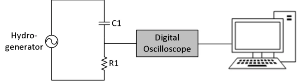
Fig. 1. Sketch of circuit for measuring and registering PD signals. The sensor is the capacitive coupler C1.
Fig. 1 shows a sketch of the measurement circuit based on the electric method. The coupling circuit
is a high-pass RC filter, whose parameters should be tuned to increase sensitivity to PD signals. It
filters the power signals and low frequency noise. The capacitor C1 is typically of 80 pF and the resistance R1 usually ranges from 500 Ω to 2000 Ω. The digital oscilloscope performs sampling and digitalization of signals and a server stores the digital data.
Other PD measurement methods have been developed in literature. The electromagnetic method,
for instance, shows the following advantages over the electric method [12]: it is non-invasive, robust
to noise and wideband.
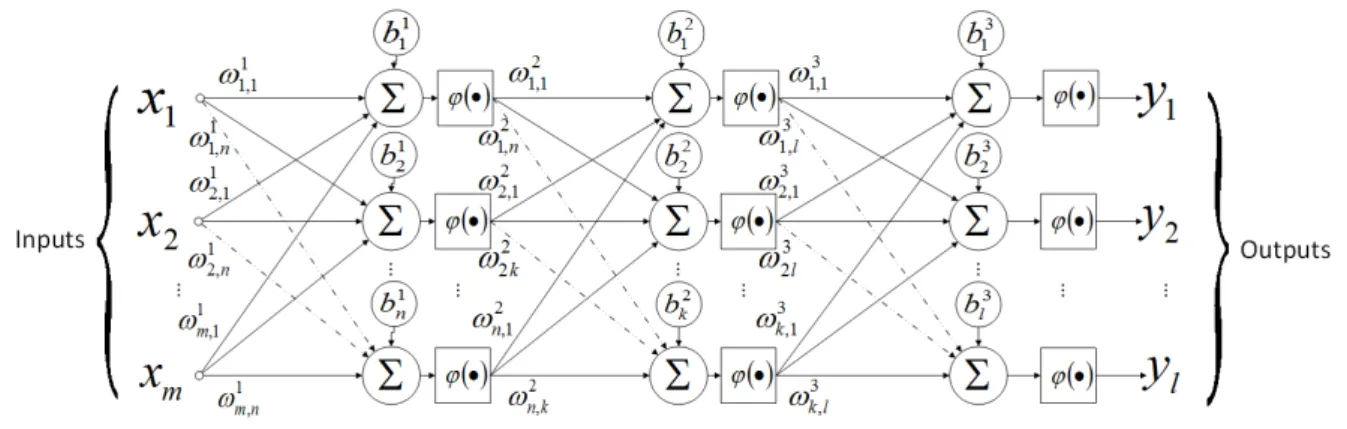
B. Artificial Neural Networks
Artificial neural networks (ANNs) are a collection of interconnected processing units which is
capable of inferring (or “learning”) relations between inputs and outputs. Their design mimics the
human brain [13].
ANN’s basic processing unit is the artificial neuron, shown in Fig. 2. The neuron applies the following mathematical operations in the inputs xi to calculate the output y:
y
i
ix
i
b
, (1)where ωi are the synaptic weights, b is the bias, which serves to increase or decrease the activation
function input, and φ is the activation function, which limits the neuron output to a predetermined
Fig. 2. Mathematical model of artificial neuron.
In order to infer more complex relations between inputs and outputs, multiple neurons are
connected in several architectures. The architecture of interest in this work is the Multilayer
Feedforward [13], shown in Fig. 3.
Fig. 3. Generic multilayer feedforward neural network.
The neural network infers the relations between inputs and outputs by means of an iterative tuning
of weights during training. In the supervised learning scheme, adopted in this work, the network is
presented to input samples with known outputs during the training phase. Such a correspondence
between inputs and outputs is generally obtained by hand labeling [13]. Once trained, a neural
network can classify, with some level of error, any sample (set of inputs) consistent with any of the
patterns to which it has been exposed during the training process. The goal is to automatically classify
samples not present in the training data set.
C. K-fold cross-validation
Evaluating the classifier performance is of fundamental importance in Machine Learning science
[14]. K-fold cross-validation (CV) allows for comparing different classifiers (and various methods)
and selecting the most suitable one for a given classification problem. In general terms, the best
classifier is the one that better generalizes the problem. Generalization is the ability of correctly and
reliably classifying samples that were not used in training. When database is limited, K-fold
cross-validation is the most used statistical technique to estimate classifier performance [14].
(folds) using stratified sampling, that is, classes in each fold are represented in approximately the
same proportion as in the data set. One fold is taken as the test set, while the others are used for
training (or training and validation, depending on the training algorithm). The error over the test fold
is calculated. This process is repeated k iterations, so that each fold has been used for testing once.
The overall error estimate is the average of the k test errors [14].
Fig. 4. K-fold cross-validation. E is the overall error estimate.
III. DATA SET
The data set used in this work is formed from online PD measurements performed in
hydro-generators at the Power Plants Tucuruí and Coaracy Nunes, both located in Northern Brazil. Fig. 5
illustrates our measurement procedure on a hydro-generator at Tucuruí.
Fig. 5. Online partial discharge measurement in a hydro-generator at Tucuruí Power Plant. Inset highlights the terminal box.
Capacitive couplers are installed close to several stator windings of the studied hydro-generators.
Employing a measurement circuit similar to that of Fig. 1, the output transient voltage signals were
Discharges (IMA-DP) [15]. This system applies several proprietary filters to the measured signal, and
stores the information about the peaks of the PD signal detected during acquisition. The rest of
time-domain signal is discarded. From the stored peaks, IMA-DP builds PRPD (Phase-Resolved Partial
Discharge) diagrams by dividing the amplitude and phase ranges in 256 windows each, resulting in
256×256 diagrams. Also referred to as φ-q-n diagrams, PRPDs are statistical maps relating the
quantity of partial discharges to their magnitude and phase of the sinusoidal wave (60 Hz). PRPDs are
considered one of the most powerful tools for PD identification [7].
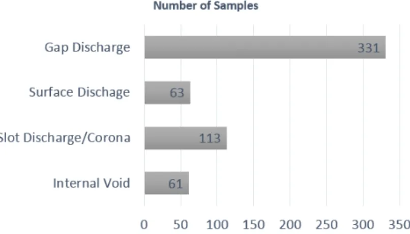
The whole data set contains 568 PRPDs measured in real hydro-generators (Fig. 5). The collected
samples were manually labeled by a human specialist among five of the most common PD sources
described in IEC 60034-27-2 [16]: internal void, slot, corona, tracking and gap discharge (Fig. 6 and
Fig. 7). Internal delamination was not considered because available samples available yielded a
certain degree of classification uncertainty: they can be easily misclassified as internal void, even by
the human expert. The delamination type, which takes place between conductor and insulation, was
also ignored due to the few samples in the data set. Also, the samples of slot and corona were merged
into a single class due to their similar PRPD characteristics [7], reducing the problem complexity. Fig.
6 shows the distribution of PD sources in the data set. It is clearly observed an imbalance among the
classes as a result of the predominance of certain PD types (classes) in the investigated machines.
Fig. 6. Distribution of PD sources in the data set.
The PRPDs in the data set present different degrees of difficulty for recognition. Some of the
samples clearly belong to their respective classes, as shown in Fig. 7. Other samples are complex, i.e.,
show ambiguity between two classes, intense noise and/or multiple PD sources (Fig. 8). Automatic
recognition of complex patterns is difficult [16], and their presence is expected due to the occurrence
of multiple simultaneous PDs sources (of different classes) in rotating machines, and due to the
Fig. 7. Examples of PRPDs from the data set. (a) Internal void. (b) Slot. (c) Corona. (d) Surface tracking. (e) Gap discharges.
Fig. 8. Examples of complex patterns from the data base: (a) gap discharges close to internal void clouds; (b) uncertainty between slot (triangular blue contour) and corona (rounded purple contour); (c) gap discharges superposed onto internal
void, as well as strong noise.
IV. THE PROPOSED CLASSIFICATION METHODOLOGY
With the methodology proposed in this work, one can perform automatic recognition of the primary
(dominant) PD source using artificial neural networks. The complete flowchart of the methodology is
shown by Fig. 9.
Three stages are considered: training, validation and testing. In the training and validation stages,
the objective is to find an optimized neural network for the PD recognition task. Specifically, during
training the optimal weights and biases of a neural network are calculated based on a subset of data,
whereas in validation the error over a second set acts as a stopping criterion of training in order to
avoid overfitting [14]. In the test stage, samples used neither in training nor in validation steps are
presented to the trained classifier in order to estimate its performance on unseen data.
treat the data with manual techniques in order to reduce the influence features from non-dominant (or
not of interest) classes (in a given sample) and/or excessively contaminated with noise that may
degrade classifier learning. Also, the time for training and validation is not critical. In all stages, the
measured samples are subjected to the same preprocessing techniques for noise treatment and
extraction of input features, producing the data effectively presented to the ANNs.
Fig. 9. Flowchart of the methodology.
A. Manual Removal of Class Ambiguities
This data cleaning technique consists of manually removing class ambiguities, i.e., partial
discharges relative to sources apart from the PD source of interest. For example, in Fig. 8(a), the
source of interest can be considered to be internal void, while gap discharges can be judged to
produce ambiguities. Removing this kind of ambiguity is necessary for the training process; otherwise
the classifier would blend different classes, reducing the training effectiveness.
After carefully inspecting the data base, all ambiguities clearly separable from the clouds of interest
have been removed. However, it is not possible to eliminate ambiguities superposed onto the main
clouds, as doing so would distort the PD pattern of interest. Clouds in PRPDs with superposed
ambiguities were kept unchanged in the data base as long as the ambiguities do not significantly
change input features regarding the PD source of interest, such as shape and symmetry.
Each row of Fig. 10 contains the results of ambiguity removal applied to the patterns of Fig. 8(a)
and Fig. 8(c), depending on which PD source is considered to be of interest. In Fig. 10(a), there is no
overlapping between gap discharges and internal void clouds. Therefore, ambiguity removal of this
Fig. 10(c). In the PRPD of Fig. 10(d), on the other hand, some gap discharges are superposed onto
internal void. In this case, all ambiguities are removed except those superposed to the primary clouds,
as shown by Fig. 10(e) and Fig.10(f). Notice that elimination of superposed PDs of different classes is
not necessary for proper ANN training since they do not significantly affect main features of PD
clouds of interest, as depicted by the filtered PRPDs of Figs. 10(e) and 10(f).
Removal of ambiguities is the only manual step in the methodology. It is automatically performed
in other works using algorithms to separate multiple simultaneous PD sources, such as clustering in
time-frequency maps [6]. However, this is not possible with PRPD maps because they are based
solely on PD peaks.
Fig. 10. Results of ambiguity removal applied to two measured PRPDs (a and d), considering that the PD source of interest is internal void (b and e) or gap discharges (c and f).
B. Removal of Sparse Partial Discharges
The patterns are then subjected to an automatic filtering by means of pixel submatrices, of which
purpose is to remove isolated PDs. Here, PRPDs are treated as negative images, whose non-black
pixels are non-zero PD counts (Fig. 11).
First, the neighborhood of each pixel is defined as the 5×5 submatrix centered in it. The filtering
consists of removing pixels that are the only nonzero in their respective neighborhoods. Fig. 11 shows
the results of such filtering applied to a PRPD from the data set.
The submatrix dimension was chosen empirically, in order to keep the algorithm conservative. With
notices in Fig. 11.
Fig. 11. PRPD (a) before and (b) after sparse PD removal by the pixel submatrix technique.
C. Feature Extraction
PRPDs from the database are 256×256 matrices, totaling 65,536 elements. Using all PRPD points
as input features would incur in a problem of very high dimensionality for ANNs. In this situation,
many features are of minor relevance, and a single point contributes very little to differentiate among
classes [14]. Therefore, it is convenient to extract from the filtered samples a subset of features of
more significance for performing the classification of the PD type.
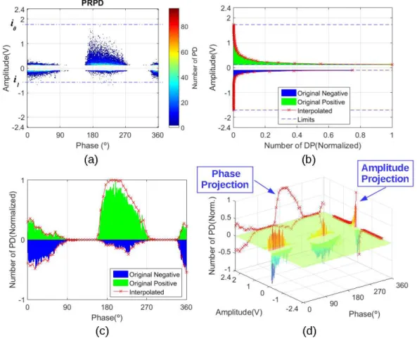
The input features used in this work are novel. They are based on the projection of normalized
PRPD counts onto the vertical (amplitude) and horizontal (phase) axes. The projections onto
amplitude and phase were calculated for each polarity separately in order to properly characterize
clouds of positive and negative PD amplitudes. This division is important to define, for example, the
presence of symmetric or non-symmetric clouds or the shape of the clouds. These features can be
determinant to properly perform PD classification [7], [16].
Given a PRPD map, the first step is to divide (normalize) all PD counts by the maximum counting
found in the map, resulting in a m × n matrix M. Normalization is necessary because it eliminates the
effect of random variables related to PD activity and measurement procedures, such as the severity of
the insulation defect and its distance to the sensor, and time of acquisition. The projections onto the
positive and negative amplitudes Pa+ and Pa-, and onto phase in positive and negative polarities Pf+
and Pf- are calculated using (2) and (3), respectively, which are given by
,
{
1
,
2
,...,
}
,
{
1
,
2
,...,
}
.
)
,
(
)
(
)
,
(
)
(
2 / 1 2 2 /1
j
n
j
i
M
j
P
j
i
M
j
P
m i m f m i f
(3)In (2) and (3), M(i, j) is the normalized quantity of PDs at magnitude i and phase j.
The amplitude range containing the relevant PRPD information is not fixed across samples. In order
to obtain this range, let i0 and i1 be the highest absolute positive and negative amplitudes. The
amplitude ranges are bounded by max(i0, i1) and -max(i0, i1), as illustrated by Fig. 12. Next, 64 points
are interpolated from both amplitude projections within the amplitude range, and 64 points are
interpolated from the phase projections in both polarities over the 60 Hz phase cycle. Fig. 12
illustrates this feature extraction procedure.
The 64 interpolated points from each of the four projections are the data effectively presented to
ANNs, totaling in 256 input features. This represents a significant dimensionality reduction.
Moreover, in Fig. 12 it can be observed that amplitude projections preserve the asymmetry between
positive and negative PDs, while phase projections indicate the cloud shape and its positioning along
the 60 Hz phase cycle. With the developed procedure, one can obtain features compatible with the PD
characteristics mentioned in IEC 60034-27-2 [16] to describe each PD type in qualitative terms,
indicating that the selected input features can, in fact, be used to classify hydro-generator PDs.
Fig. 12. Feature extraction. Input features are red points. (a) PRPD. (b) Projections onto amplitude. (c) Projections onto phase. (d) PRPD surface representation in 3-D space along with the amplitude and phase projections, which are perceived to
D. Training and Validation of Neural Networks
Neural networks were trained in such a way to reduce the influence of ANN topology and of the
following random variables: data sampling and initial weights. The topology (number of hidden layers
and number of neurons per hidden layer) is a free parameter of neural networks, and its optimal
configuration is not known beforehand. For this reason, ANNs of several topologies were trained. In
order to mitigate potential performance inclinations due to the particular distribution of data that
compose the training, validation and test sets, each topology was trained with several partitions of the
data, using the strategy of stratified 4-fold cross-validation (CV) [14], repeated 10 times. Each CV
partition consists of selecting two folds to form the training set, one for validation and the other for
testing. The 12 possible partitions are considered for each repetition of cross-validation.
In a given partition, the training samples are presented to the ANN, and its weights and biases are
updated iteratively in this work by means of the Scaled Conjugate Gradient Backpropagation
algorithm (SCG) [17]. The validation error is calculated. In order to avoid overfitting [14], this
process is repeated until the validation error starts to increase. Once trained, the neural network
classifies the test set, and the resulting error is used to estimate the error over unknown samples (see
Section V).
Initial weights have a major influence on training. The training of neural networks is a complex
optimization problem. The goal is to find the combination of weights/biases (solution) that minimizes
the difference (error function) between the ANN output and target classes. From a random guess, the
SCG algorithm moves the solution iteratively in the direction of the negative of the error function
gradient, converging to the closest point with zero gradient. Since the error function is generally
non-convex and multimodal [13], gradient-based algorithms tend to get “stuck” at the closest local
minimum. Initial solutions are totally random parameters, and the convergence to local optima is a
characteristic of the training algorithm.
In order to mitigate the mentioned influence of the initial values of network weights on training, for
each topology, 50 ANNs of different initial weights (defined randomly) were trained in each CV
partition. Moreover, all ANNs have 256 input neurons, 4 output neurons, hyperbolic tangent
activation function in hidden layers and softmax function in output layer.
V. RESULTS AND DISCUSSION
A. Analysis of ANN recognition performances
Considering the training and validation stages, as described in Section IV (Fig. 9), the patterns were
noise-filtered and its features extracted. Then, such features were used as inputs of neural networks.
All the trained ANNs were evaluated one by one in the following way. Each ANN is executed over
the test fold relative to the CV partition in which it was trained. For each of the C classes, it is
calculated the true positive rate per class (TS), which is equal to the rate of samples of a given class
Cj i j i i Si
n
n
T
1 , ,, (4)
where ni,j is the number of samples known to be of class i but predicted to be of class j. Then, we
calculate the average
Ts and standard deviation
Ts of the C true positive rates per class:
C i Si TsT
C
11
(5)and
Ci Si Ts
Ts
T
C
12
1
. (6)The recognition performance of each ANN is quantified by the novel metric δ, defined as:
Ts Ts
1
1
. (7)
As observed in Equation (7), δ has two contributions: one increases with
Ts and the otherdecreases with
Ts. The first term is associated to the classifier’s average performance across classes.The second term accounts for the variability of true positive rates per class. It distinguishes classifiers
with similar
Tsby ranking higher those with more uniform success rates across classes (less biased).The idea of δ is to appropriately rank classifiers that perform similarly well at recognizing samples of different classes. Thus, a desirable classifier is that with high recognition rates for any class (high
Ts
), with rates that do not differ much from one another (low
Ts).Global success rate (rate of correctly classified samples relative to the size of the data set), a
typically used criterion for evaluating classifiers [14] , is not suitable for problems with imbalanced
data sets because it is biased towards the classes with most samples. Also, since δ is calculated over
samples not used in training (test set), it estimates a classifier’s generalization capabilities. It is worth
mentioning that δ is a generic metric; it can be used to evaluate any classifier in any Machine
Learning application involving the recognition of a single class per sample.
In the following results, the neural network topology is expressed as the number of hidden neurons
separated by dashes. NHL is the topology with no hidden layers: inputs are directly connected to
output neurons. In addition, due to the fact that the initial weights are not related to the classification
problem itself (Section IV.D), their influences are minimized by showing results for the 25% best
neural networks of each topology.
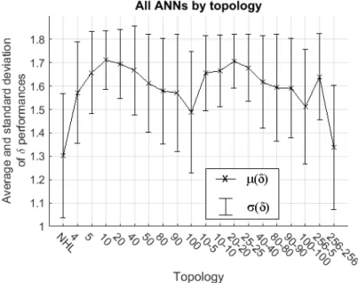
Fig. 13 contains the average μ(δ) and standard deviation σ(δ) of δ performances of all ANNs of
measure the influence of topology on performance, after varying initial weights and CV partitions.
Fig. 13. Average (line) and standard deviation (vertical bars) of δ performances of all networks for each topology. Vertical bars are the size of two standard deviations.
Fig. 14. Average (line) and standard deviation (vertical bars) of δ performances of the 25% best networks of each topology. Vertical bars are the size of two standard deviations.
Similar interpretation of δ is used to rank the different topologies: the best topologies are those whose networks present high average performances (high μ(δ)) and low standard deviation (σ(δ)) for the obtained values of δ. It is worth mentioning that μ(δ) and σ(δ) are different than
Ts and
Tsfrom(5) and (6), respectively. The latter two indicate the variation of performance across classes, and are
calculated for each network in order to calculate its performance δ. The former two, on the other hand,
select the most suitable topology (which is a free parameter of ANNs) for the problem at hand.
In Fig. 14, due to the reduced influence of random initialization of weights, one can observe that the
average and standard deviation of δ are relatively constant over the range between topologies 50 and
256-5. Topologies 10, 20 and 40 presented larger μ(δ) and similar σ(δ). The worst performance was
observed for NHL (low average and large standard deviation of δs), indicating that the use of hidden
layers is important to capture the non-linear relations between inputs and outputs. Similar observation
was made in [9]. Bad results were also obtained for topology 256-256, probably because the number
of samples was insufficient to train a network with so many weights and biases. Topology 10 is
considered to be the most favorable on average, because it is the simplest configuration (low number
of weights) of which most networks presented good generalization (high average and low dispersion
of values of δ).
The curve in Fig. 13 presents higher variation in average δ across topologies, as well as much
higher standard deviation due to random weight initialization influence. The poorer results are due to
networks trained from inappropriate initial weights. Even with those differences, the best and worst
topologies are the same as those mentioned above for Fig. 14, showing the representativeness of the
25% best networks in relation to all networks.
The next results are relative to the most favorable topology 10, and are illustrated by means of
confusion matrices. A confusion matrix shows classification results intuitively [14]. Rows and
columns are relative to true and predicted classes, respectively. Element (i,j) is equal to the number of
samples known to be of class i classified as being of class j. Evidently, the correct classifications are
evaluated by the elements in main diagonal.
To obtain a picture of average performance of all networks of topology 10, their confusion matrices
over the test set were summed element-wise. Each element was calculated as the percent ratio relative
to the sum in the respective row, resulting in the matrix shown in Fig. 15.
Fig. 16. Element-wise average confusion matrix of the 25% best ANNs of topology 10 over the test set.
The same is performed in Fig. 16 for the 25% best networks of topology 10. In Fig. 16, the
interpretation for element (1,3), for example, is that 6.20% of internal void samples were misclassified
as tracking by the best networks, on average. The classes with the highest success rates were
slot/corona and gap discharges, probably because these are the classes with the highest number of
samples (Fig. 6). Smaller success rates were obtained for the other classes, indicating that the
methodology can be worse at recognizing internal void and tracking patterns. Tracking samples are
primarily misclassified as gap, while the inverse happens in a reduced degree. Confusion between
tracking and gap discharges is reasonable, as these are the only classes formed by clouds of discharges
far from the central region of PRPD. The same conclusions can be drawn from Fig. 15. The
differences between these two Figures – also caused by suboptimal initial weights – are lower
recognition rates and consequently more frequent misclassifications.
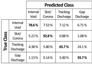
The primary goal is to find an optimized network for trustworthy classifying PDs. Fig. 17 shows the
confusion matrix of the best neural network (largest δ) of topology 10 over the test set. High
recognition rates (of at least 94%) were obtained for all classes.
B. Graphical User Interface
A graphical user interface (GUI) was developed in order to display in an interactive way the results
of PD classification and to automate the classification process. The classification is performed by a
previously trained ANN by executing the test stage shown in Fig. 9.
The developed interface is shown in Fig. 18. It displays, from left to right, the PRPD of current
sample, amplitude and phase projections, and pertinence probabilities of the current sample to the
different classes. Pertinence probabilities are proportional to the ANN outputs. The final PD
classification – the class with the highest pertinence – is shown in the lower right corner.
Fig. 18. The graphical user interface (GUI) developed in this work to aid in decision making. Pattern was correctly classified as internal void.
Understanding the interface’s intuitive indications does not require specialized operators, reducing training and operational costs and facilitating the application of the methodology in a real monitoring
system by non-specialized human operators.
VI. FINAL REMARKS
In this work, a methodology for automatic partial discharge classification using neural networks is
presented. The neural networks were trained to classify a single PD source using novel features
extracted from PRPD maps.
Several networks were trained, and their performances were assessed and compared statistically.
Topology with 1 hidden layer and 10 hidden neurons was found to be the most favorable on average.
The best network obtained presented very good performance. PD sources slot/corona and gap
discharge were the classes most correctly classified among the networks.
classifying multiple PD sources. Considering all PD sources described in standards and solving the
issues of similarities between slot and corona are problems of great interest.
REFERENCES
[1] G. Stone. A perspective on Online Partial Discharge Monitoring for Assessment of the Condition of Rotating Machine Stator Winding Insulation. IEEE Electrical Insulation Magazine, vol. 28, no. 5, pp. 8-13, 2012.
[2] G. Stone. Partial Discharge Diagnostics and Electrical Equipment Insulation Condition Assessment. IEEE Transactions on Dielectrics and Electrical Insulation, vol. 12, no. 5, pp. 891-904, 2005.
[3] G. Stone and V. Warren. Objective Methods to Interpret Partial-Discharge Data on Rotating-Machine Stator Windings. IEEE Transactions on Industry Applications, vol. 42, no. 1, pp. 195-200, 2006.
[4] N. Malik and A. Al-Arainy and M. Qureshi. Electrical Insulation in Power Systems. Marcel Dekker, 1998.
[5] R. Bartnikas. Partial Discharges: Their Mechanism, Detection and Measurement. IEEE Transactions on Dielectrics and Electrical Insulation, vol. 9, no. 5, pp. 763-808, 2002.
[6] IEC TS 60034-27. Rotating electrical machines - Part 27: Off-line partial discharge measurements on the stator winding insulation of rotating electrical machines. International Electrotechnical Commission, 2006.
[7] C. Hudon and M. Bélec. Partial Discharge Signal Interpretation for Generator Diagnostics. IEEE Transactions on Dielectrics and Electrical Insulation, vol. 12, no. 2, pp. 297-319, 2005.
[8] J. Tang and F.Liu and Q. Meng and X. Zhang and J. Tao. Partial Discharge Recognition through an Analysis of SF6
Decomposition Products Part 2: Feature Extraction and Decision Tree-based Pattern Recognition. IEEE Transactions on Dielectrics and Electrical Insulation, vol. 19, no. 1, pp. 37-44, 2012.
[9] H. Ma and J. Chan and T. Saha and C. Ekanayake. Pattern Recognition Techniques and Their Applications for Automatic Classification of Artificial Partial Discharge Sources. IEEE Transactions on Dielectrics and Electrical Insulation, vol. 20, no. 2, pp. 468-478, 2013.
[10]H. Sinaga and B. Phung and T. Blackburn. Recognition of single and multiple partial discharge sources in transformers based on ultra-high frequency signals. IET Generation, Transmission Distribution, vol. 8, no. 1, pp. 160-169, 2014.
[11]IEC 60270. High-voltage test techniques - Partial discharge measurements. International Electrotechnical Commission, 2000.
[12]V. Dmitriev and R. M. S. Oliveira and F. Brasil and P. Vilhena and J. Modesto and R. Zampolo. Analysis and Comparison of Sensors for Measurements of Partial Discharges in Hydrogenerator Stator Windings. Journal of Microwaves, Optoelectronics and Electromagnetic Applications, vol. 14, no. 2, pp. 197-218, 2015.
[13] S. Haykin. Neural Networks - A comprehensive foundation. 2nd ed. Prentice Hall, 2004.
[14]I. Witten and E. Frank and M. Hall. Data Mining: Practical Machine Learning Tools and Techniques. 3rd ed. Morgan Kaufmann, 2011.
[15]H. Amorim and A. Carvalho and O. Fo. and A. Levy and J. Sans. Instrumentation for Monitoring and Analysis of Partial Discharges Based on Modular Architecture, in International Conference on High Voltage Engineering and Application (ICHVE 2008), pp. 596-599, 2008.
[16]IEC 60034-27-2. Rotating electrical machines - Part 27-2: On-line partial discharge measurements on the stator winding insulation of rotating electrical machines. International Electrotechnical Commission, 2012.