Modeling and numerical simulation of fluid flow and heat transfer of a steel continuous casting tundish

UNIVERSIDADE FEDERAL DO CEARÁ CENTRO DE TECNOLOGIA

DEPARTAMENTO DE ENGENHARIA METALÚRGICA E DE MATERIAIS PROGRAMA DE PÓS-GRADUAÇÃO EM ENGENHARIA E CIÊNCIA DE

MATERIAIS

JOSÉ RENÊ DE SOUSA ROCHA

MODELING AND NUMERICAL SIMULATION OF FLUID FLOW AND HEAT TRANSFER OF A STEEL CONTINUOUS CASTING TUNDISH

MODELING AND NUMERICAL SIMULATION OF FLUID FLOW AND HEAT TRANSFER OF A STEEL CONTINUOUS CASTING TUNDISH

Dissertação submetida ao Programa de Pós-Graduação em Engenharia e Ciência de Materiais da Universidade Federal do Ceará como requisito parcial à obtenção do título de Mestre em Engenharia e Ciência de Materiais. Área de Concentração: Processos de transformação e degradação dos materiais.

Orientador: Prof. Dr. Francisco Marcondes

Gerada automaticamente pelo módulo Catalog, mediante os dados fornecidos pelo(a) autor(a)

R573m Rocha, José Renê de Sousa.

Modeling and numerical simulation of fluid flow and heat transfer of a steel continuous casting tundish / José Renê de Sousa Rocha. – 2017.

91 f. : il. color.

Dissertação (mestrado) – Universidade Federal do Ceará, Centro de Tecnologia, Programa de Pós-Graduação em Engenharia e Ciência de Materiais, Fortaleza, 2017.

Orientação: Prof. Dr. Francisco Marcondes.

MODELING AND NUMERICAL SIMULATION OF FLUID FLOW AND HEAT TRANSFER OF A STEEL CONTINUOUS CASTING TUNDISH

Dissertação submetida ao Programa de Pós-Graduação em Engenharia e Ciência de Materiais da Universidade Federal do Ceará como requisito parcial à obtenção do título de Mestre em Engenharia e Ciência de Materiais. Área de Concentração: Processos de transformação e degradação dos materiais.

Aprovada em: 17/02/2017.

BANCA EXAMINADORA

________________________________________ Prof. Dr. Francisco Marcondes (Supervisor)

Federal University of Ceará (UFC)

_________________________________________ Prof. Dr. Clovis Raimundo Maliska

Federal University of Santa Catarina (UFSC)

_________________________________________ Prof. Dr. Janaína Gonçalves Maria da Silva Machado

Federal University of Ceará (UFC)

_________________________________________ Dr. Eng. Alex Maia do Nascimento

To God.

First of all, I would like to thank my family, specially my parents, Pedro and Celina, for all support during these years that I have been at Federal University of Ceará, for their good advices and guidance to succeed in all steps of my life.

I am thankful to all professors who I had the opportunity to study during these two years at the Graduate Program in Engineering and Material Science, besides, I would also like to express my gratitude for their help and effort to transmit some fundamental knowledge to us. Amongst the professors, I would like to thank my supervisor, Francisco Marcondes, with whom I had the opportunity to develop this study. In addition, I thank him for his fundamental experience during the supervision of this research, his helpful tips and review of this text, and all his collaboration during the development of this thesis.

I am also grateful to the committee members, composed by prof. Dr. Francisco Marcondes, prof. Dr. Clovis Raimundo Maliska, prof. Dr. Janaína Gonçalves Maria da Silva Machado, and Dr. Eng. Alex Maia do Nascimento, for their availability in being part of this work.

I would like to thank my classmates and friends for the great moments of joy and studies throughout this long journey of hard work. Furthermore, I would like to recognize the great advices, comments, and the significant sharing of information that I have received from my friends from the Computational Fluid Dynamics Laboratory (LDFC) and especially thank to Ivens, whose guidance at earlier stages of this thesis brought some fundamental contribution to this work to be finished.

“We should all be concerned about the future because we will have to spend the rest of our lives there.”

Currently, the continuous casting process is the most used technique to produce steel. Being an inherently component of the caster machine, the tundish has been designed to be not only an intermediate vessel between the ladle and the mold, but also a device to remove inclusions and a metallurgical reactor. Therefore, the tundish has an important role in the continuous casting process. The physical model for heat transfer and fluid flow into the tundish is very complex, thus analytical solutions are not available. Physical studies might present many difficulties for analyzing the process. Hence, Computational Fluid Dynamics (CFD) emerges as an attractive alternative. CFD is based on numerical approaches that are used to solve several classes of engineering problems. The main goal of the present study is to analyze the fluid flow and temperature fields into an actual tundish configuration that is used in continuous casting processes of a local steelmaker company. Based on the performed simulations, some modifications in the geometry of the tundish are proposed in order to improve the steel quality; these modifications make use of weirs and dams. For solving the governing equations arising from the physical model, the Ansys CFX software, which is based on the Element-based Finite-Volume Method (EbFVM) were used. Simulations were performed using water and steel as working fluids for a turbulent flow in a 3D tundish. The results were presented in terms of velocity and temperature fields and Residence Time Distribution (RTD) curves, which evaluated them qualitatively and quantitatively.

O processo de lingotamento contínuo é o processo mais utilizado na produção de aço atualmente. Sendo um importante componente da máquina de lingotamento, o distribuidor tem sido projetado para atuar não apenas como um reservatório entre a panela e o molde, mas também como um dispositivo para remoção de inclusões e servir como um reator metalúrgico. Logo, o distribuidor assume um papel de relevância no processo de lingotamento contínuo. O modelo físico que rege a transferência de calor e escoamento dentro do distribuidor apresenta grande complexidade, tornando a sua solução analítica indisponível. Estudos físicos podem apresentar várias dificuldades para a análise do processo. Portanto, a Dinâmica dos Fluidos Computacional (CFD) surge com uma alternativa viável. CFD é baseada em aproximações numéricas as quais são utilizadas para a solução de várias classes de problemas de engenharia. O principal objetivo do presente trabalho é analisar os campos de escoamento e temperatura no interior de um distribuidor o qual é utilizado nos processos de lingotamento contínuo de uma companhia siderúrgica local. Com base nas simulações realizadas, modificações na geometria do distribuidor são propostas com o intuito de aumentar a qualidade do aço. Essas modificações são feitas através do uso de diques e barragens. Para a solução das equações de conservação originadas do modelo físico, o programa Ansys CFX, o qual utiliza o Método dos Volumes Finitos baseado em Elementos (EbFVM), foi utilizado. As simulações foram feitas utilizando-se aço e água como fluidos de trabalho para um escoamento turbulento em um distribuidor tridimensional. Os resultados foram apresentados em termos de campos de velocidade e temperatura e curvas de Distribuição de Tempo de Residência (RTD) as quais serviram para analisá-los qualitativa e quantitativamente.

Figure 1.1 - Fraction of steel produced by continuous casting process in the last decades...

18

Figure 2.1 - Schematic of steel continuous casting process... 22

Figure 2.2 - Flow control modifiers (dams and weirs)... 27

Figure 2.3 - Typical RTD (Residence Time Distribution) curves for different tundish configurations………... 27

Figure 2.4 - Temperature contour on longitudinal plane... 29

Figure 2.5 - Comparison between isothermal and non-isothermal RTD curves... 29

Figure 2.6 - Inclusion removal for isothermal and non-isothermal models... 31

Figure 2.7 - Unstructured mesh and control-volume... 32

Figure 2.8 - Combined model... 37

Figure 2.9 - Fluid flow crossing the active and dead regions in a combined model…... 37

Figure 2.10 - Tundish volume regions... 40

Figure 3.1 - Work methodology... 42

Figure 4.1 - Inclusion removal with and without the Random Walk model... 49

Figure 5.1 - Cross section of a mesh for case I... 57

Figure 6.1 - Comparison with experimental data for validation case II. (a) Central exit nozzle (b) Lateral exit nozzle... 58 Figure 6.2 - Comparison with numerical data with no RWM…... 60

Figure 6.3 - Comparison with numerical data with RWM... 60 Figure 6.4 - Isothermal flow pattern for case study I. (a) At the inlet longitudinal plane.

(b) At the outlet longitudinal plane. (c) At the inlet transverse symmetry plane...

62 Figure 6.5 - Isothermal flow pattern for case study II. (a) At the inlet longitudinal plane.

(b) At the outlet longitudinal plane. (c) At the inlet transverse symmetry plane...

64 Figure 6.6 - Isothermal flow pattern for case study III. (a) At the inlet longitudinal

plane. (b) At the outlet longitudinal plane. (c) At the inlet transverse symmetry plane...

65 Figure 6.7 - Comparison of the three cases – Isothermal analysis. (a) RTD curves for

the whole simulation time. (b) RTD curves showing the concentration peaks...

analysis... 69 Figure 6.9 - Temperature contours for case study I. (a) At the inlet longitudinal plane.

(b) At the outlet longitudinal plane. (c) At the inlet transverse symmetry plane...

70 Figure 6.10 - Temperature contours for case study II. (a) At the inlet longitudinal plane.

(b) At the outlet longitudinal plane. (c) At the inlet transverse symmetry plane...

71 Figure 6.11 - Temperature contours for case study III. (a) At the inlet longitudinal plane.

(b) At the outlet longitudinal plane. (c) At the inlet transverse symmetry plane...

73 Figure 6.12 - Comparison of the three cases – Non-isothermal analysis. (a) RTD curves

for the whole simulation time. (b) RTD curves showing the concentration peaks...

74 Figure 6.13 - Lagrangian analysis for the three cases with RWM – Non-isothermal

analysis... 76 Figure A.1 - Geometry and surface mesh for Case I... 86 Figure A.2 - Geometry and surface mesh for Case II... 86 Figure A.3 - Geometry and surface mesh for Case III... 87 Figure A.4 - Geometry and surface mesh for the validation case I (Kemeny et al., 1981)

... 87 Figure A.5 - Geometry and surface mesh for the validation cases II and III (Wollmann

Table 2.1 – Physical properties of water at 20ºC and liquid steel at 1600ºC... 24

Table 2.2 – Steel cleanliness requirements for maximum inclusion size... 25

Table 2.3 – Turbulence models... 34

Table 5.1 – Physical and operating parameters for validation cases... 52

Table 5.2 – Physical parameters for case studies... 53

Table 5.3 – Operating parameters for case studies... 53

Table 5.4 – AISI 1025 steel thermophysical properties... 54

Table 5.5 – Number of nodes used for each case study... 56

Table 6.1 – Comparison with experimental and numerical analyses – Validation case I... 57

Table 6.2 – Comparison with experimental and numerical analyses – Validation Case II... 59

Table 6.3 – Minimum and mean residence time for each configuration – Isothermal analysis... 68

Table 6.4 – Volume fraction of flow – Isothermal analysis... 68

Table 6.5 – Minimum and mean residence time for each configuration – Non-isothermal analysis... 75

AISI American Iron and Steel Institute CFD Computational Fluid Dynamics.

CNPq National Council of Technological and Scientific Development (Conselho Nacional de Desenvolvimento Científico e Tecnológico) DNS Direct Numerical Simulation

EbFVM Element-based Finite-Volume Method FDM Finite Difference Method

FEM Finite Element Method FVM Finite Volume Method LDA Laser Doppler Anemometer LES Large Eddy Simulation.

RANS Reynolds Averaged Navier-Stokes RMS Root Mean Square

1

a Constant for SST turbulence model.

C Dimensionless concentration.

D

C Drag coefficient.

p

C Specific heat at constant pressure, [ J kg .K ].

1

C_ Constant for k turbulence model.

2

C_ Constant for k turbulence model.

C_ Constant for k turbulence model.

D Kinematic diffusivity.

eff

D Effective kinematic diffusivity.

p

d Diameter of the particle, [kg m3].

1

F Blending function for SST turbulence model.

2

F Blending function for SST turbulence model.

g _{Gravitational acceleration, [} 2 m s ].

h _{Enthalpy, [} 2 2

m s ].

h _{Heat transfer coefficient, [} 2

W m .K].

K _{Thermal conductivity, [W m.K ].}

eff

K Effective thermal conductivity, [W m.K ].

k _{Turbulence kinetic energy, [} 2 2

m s ].

p

m Mass particle, [ kg ].

t

m Tracer mass, [ kg ].

p _{Pressure, [} 2

N m ].

Pr Turbulent Prandtl number.

k

P Turbulence production, [kg m.s3].

Re Reynolds number.

S Invariant measure of the strain rate.

c

S Turbulent Schmidt number.

q Heat flux, [W m ].

q Volumetric flow rate, [m s3 ].

T Temperature, [K].

ref

T Reference temperature, [K].



T Room temperature, [K].

t Theoretical residence time, [s].

min

t Minimum residence time, [s].

peak

t Maximum residence time, [s].

j

U Fluid velocity, [ m s ].

p

U Velocity particle, [ m s ].

V _{Tundish volume, [} 3

m ].

D

V Dead volume.

M

V Well-mixed volume.

P

V Dispersed plug volume.

3

 Constant for SST turbulence model.



'

 Constant for SST turbulence model.

3

 Constant for SST turbulence model.  Emissivity.

 Turbulence eddy dissipation, [m s2 3].  Dimensionless residence time.

min

 Dimensionless minimum residence time.

peak

 Dimensionless maximum residence time.  Dimensionless mean residence time.

C

 Dimensionless mean time from  0 to  2.  _{Dynamic viscosity, [ kg m.s ].}

eff

 Kinematic viscosity, [m s2 ].

t

 Turbulent viscosity, [m s2 ].  _{Fluid density, [} 3

kg m ].

p

 Density of the particle, [kg m3].

ref

 Reference density, [kg m3].  Stefan-Boltzmann constant.

k

 Constant for k turbulence model.

3 k

 Constant for SST turbulence model.



 Constant for k turbulence model.

3 

1 INTRODUCTION... 18

1.1 Objectives... 20

1.1.1 General objective... 20

1.1.2 Specific objectives... 20

1.1.3 Structure of the present work... 21

2 LITERATURE STUDY... 22

2.1 The continuous casting process... 22

2.2 The steel continuous casting tundish... 23

2.3 Non-metallic inclusions... 25

2.4 Flow control modifiers... 26

2.5 Thermal analysis applied to tundish modeling... 28

2.6 Numerical methods applied to tundish modeling... 31

2.7 Turbulence models... 33

2.8 RTD (Residence Time Distribution) analysis... 36

3 METHODOLOGY... 42

4 MATHEMATICAL FORMULATION... 43

4.1 Mass and momentum equations... 43

4.2 Turbulence models... 44

4.2.1 kturbulence model... 44

4.2.2 SST turbulence model... 45

4.3 Thermal energy equation... 47

4.4 Tracer convection-diffusion equation... 47

4.5 Particle tracking equation... 48

4.6 Initial and Boundary conditions... 50

5 NUMERICAL MODELING... 52

5.1 Physical and operating parameters for all cases... 52

5.2 Solution procedure... 53

5.3 Assumptions... 54

5.4 Independence tests for grid, time, and number of injected particles... 55

6.1.2 Validation case II... 58

6.1.3 Validation case III... 59

6.2 Case studies for isothermal analysis... 61

6.2.1 F low field for the three case studies... 61

6.2.2 RTD parameters for the three case studies... 67

6.2.3 Lagrangian analysis for the three case studies... 68

6.3 Case studies for non-isothermal analysis... 69

6.3.1 Temperature field for the three case studies... 69

6.3.2 RTD parameters for the three case studies... 74

6.3.3 Lagrangian analysis for the three case studies... 75

7 CONCLUSION AND FUTURE WORK... 77

7.1 Future work... 78

REFERENCES... 79

APPENDIX A – GEOMETRIES AND MESHES... 86

APPENDIX B – MESH REFINEMENT STUDY... 89

APPENDIX C – TIMESTEP CONVERGENCE STUDY………... 90 APPENDIX D – INDEPENDENCE TEST FOR PARTICLES INSERTED

AT INLET

1 INTRODUCTION

The continuous casting process transforms the liquid metal into a solid. In contrast to conventional form of steelmaking, where the molten steel is poured into a closed mold, which causes the interruption of the process every time the mold is completed, the continuous casting process occurs in a continuous basis; this is possible owing to the use of an opened mold.

The continuous casting process has many advantages over the traditional one, such as higher quality and higher productivity of molten metal, which gives it preference when low cost and high efficiency are sought in industry. Therefore, these advantages make this process the most used technique to produce steel currently. Fig. 1.1 illustrates the worldwide growing development of steel produced by continuous casting process.

Figure 1.1 – Fraction of steel produced by continuous casting process in the last decades.

Source: World Steel Association (2015).

As can be seen from Fig. 1.1, nowadays continuous casting process is responsible for producing over 96% of steel in the world. Accordingly, the full comprehension about what happens into the main devices being part of this process is of vital importance to further design and optimize it.

to maintain the ladle exchange without interrupt the process and to keep the liquid metal’s height into the mold constant.

With the aim to increase the steel quality, some flow control devices have been added to the tundish, and therefore the flow pattern may change. The most common flow modifiers include dams, weirs, stopper rods, turbulence inhibitors, baffles, and gas injectors.

Considering the importance of liquid steel to metallurgy industry, several researchers have carried out investigations in both experimental and numerical area, concerning the main relevant aspects that govern the fluid flow and heat transfer into the tundish (Gardin et al., 2002; Kumar et al., 2004). As we know, experimental analysis has many drawbacks, such as high cost of equipment and less possibility to both change and analyze different scenarios. On the other hand, performing numerical analysis of continuous casting processes can overcome these drawbacks.

The long-stablished methods to solve the partial differential equations numerically can be divided into three main categories: Finite-Volume Method (FVM), Finite Element Method (FEM), and Finite Difference Method (FDM). Moreover, Finite-Volume Method is the most used method in the commercial packages, since it is the only approach that can warrant local conservation of the physical quantities (mass, momentum, and energy) (Maliska, 2004).

Based on numerical approaches, Computational Fluid Dynamics (CFD) can be defined as the analysis of systems that involve fluid flow, heat transfer, and related phenomena such as combustion processes. In addition, solution is obtained in a computer-based simulation. CFD is based on the approximate solution of governing equations, viz., mass, momentum, and energy equations along with proper initial and boundary conditions. Also, CFD has gained great attention in the research community as a result of its flexibility and high cost-effective processes.

To perform a CFD simulation, four main steps must be followed: • Defining the geometry and creating the mesh;

• Defining the physical model; • Solving the given CFD problem; • Visualizing the obtained results.

to perform a CFD analysis. To discretize the transport equations, the Element-based Finite-Volume Method (EbFVM) is used.

Analyzing the various physical and geometric parameters involved in tundish modeling might be a complex task, especially when experimental techniques are applied. However, CFD gives rise to an easier way to deal with this task by combining numerical and computational tools. There are many advantages when comparing CFD techniques with experimental approaches, for instance, reduction of time to analyze systems with no added expenses, possibility to perform studies under hazardous conditions, infinite level of parametric studies leading to unlimited possibilities, reliable results, and ability to simulate ideal and realistic relevant problems. Nevertheless, to take full advantage of CFD capabilities, experience and exhaustive trial-and-error analysis is required by the design engineer.

However, numerical simulation in steel continuous casting tundishes should not replace experimental analysis, instead, numerical analysis must complement it in order to make integrated analysis in complex systems of vital importance to engineering.

1.1 OBJECTIVES

1.1.1 General objective

The main objective of this study is to evaluate qualitatively and quantitatively the flow field and heat transfer within a steel continuous casting tundish of a local steelmaker company.

1.1.2 Specific objectives

The main objective may be split into the following specific objectives: • Assess the velocity and temperature fields into the tundish;

• Through RTD (Residence Time Distribution) analysis, estimate time parameters (minimum and mean residence times) and the proportions of dead, dispersed plug, and well-mixed volumes;

• Estimate the proportion of removed non-metallic inclusions at slag layer; • Validate the numerical methodology using experimental works from the

• Evaluate the influence of flow modifiers (that is, dams and weirs) upon the liquid steel flow and their efficiency in making the liquid steel cleaner.

1.1.3 Structure of the present work

In the present work, a numerical modeling of a steel continuous casting tundish was performed. Eulerian and Lagrangian based analysis using both isothermal and non-isothermal models were studied. Also, two turbulence models, namely, the k model (Launder and Spalding, 1974) and SST model (Menter et al., 2003), were tested. The remainder of this work is divided in the following chapters.

Chapter 2 provides a literature study, where a detailed analysis of the relevant aspects concerning tundish modeling is presented.

Chapter 3 briefly describes the work methodology, showing each step developed in the present study.

Chapter 4 shows the mathematical model for obtaining the flow field, heat transfer, and particle path into the tundish. Also, initial and boundary conditions are shown.

Chapter 5 presents important considerations, such as physical and operating parameters, main assumptions, and solution procedure.

Chapter 6 provides the results obtained in the simulations along with some discussions of the results.

2 LITERATURE STUDY

2.1 The continuous casting process

The continuous casting process was conceived by Henry Bessemer in the 19th century. However, this process became widespread in 1960s only (Thomas, 2001b). The aforementioned process has not only been used to produce steel worldwide, but also some other basic metals have made use of it, including aluminum, copper, and nickel.

The main components of continuous casting machine, which are shown in Fig. 2.1, are listed below:

• Ladle; • Tundish; • Mold;

• Support rolls;

• Cooling spray nozzles.

Figure 2.1 – Schematic of steel continuous casting process.

According to Thomas (2001b), this process is described as follows: The steel, previously melted in a furnace is poured into a ladle. Then, molten steel is brought into the tundish through a shroud. The tundish distributes the liquid steel through the submerged entry nozzle into the mold. To protect against undesirable oxidation due to exposure to air, a slag layer is kept on the top of liquid steel of all vessels. Also, the nozzles used between the ladle, tundish, and mold need to be protected through the use of ceramic materials. In the mold, which is water-cooled, the solid shell begins to form. Drive rolls, running at a constant rate remove the solid shell from the mold. Furthermore, rolls must protect the solid steel from ferrostatic pressure. Water-air mixture sprays cool the strand surface to reduce its temperature until the steel core is fully solidified. Finally, reaching the metallurgical length, steel solidification is completed and the strand can be cut into slabs by making use of a torch.

The present work focus only on tundish; since this continuous casting component it is considered to be the last chance to make the steel cleaner before the solidification begins. In addition, it serves as a refining vessel to float out inclusions into the slag cover (Chakraborty and Sahai, 1992).

2.2 The steel continuous casting tundish

As previously pointed out, tundish plays a relevant role in continuous casting process. Its role has evolved from a simple reservoir to being a grade separator, an inclusion removal device, and a metallurgical reactor. Several tundish designs have as their aim the change in flow patterns to either achieve minimum mixed-grade length during grade transition or to increase inclusion particle removal at the slag layer (De Kock, 2005).

Once inclusion particles remain into liquid steel, they may produce local internal stress concentration, which would cause reduction in the steel fatigue life (Thomas, 2001b). As an alternative to the traditional used flow modifiers, such as dams and weirs to obtain inclusion removal, some authors have proposed the use of gas injection to improve the entrapment of non-metallic inclusions by slag layer (Jun et al., 2008; Kruger, 2010; Mendonça, 2016).

Even with enormous amounts of results that can be obtained by numerical modeling studies, they are practically useless without validations. Therefore, to provide confidence on numerical results, physical modeling studies must be carried out.

In order to represent the fluid flow of molten steel into tundish through experimental analysis, reduced or full-scale water models can be used. Nonetheless, for truly characterize the fluid flow, some conditions of similarities between the model and the actual tundish need to be satisfied. The similarities are divided into geometric, mechanical, chemical, and thermal ones. In an aqueous reduced scale model, geometrical and mechanical similarities must be attempted. To meet geometrical similarity, all dimensions must obey a specific relation between scaled model and actual tundish, whereas mechanical similarity is achieved by keeping the same forces on model and actual tundish through the Froude number (inertial forces/gravitational forces), since it is difficult to maintain both Reynolds (inertial forces/viscous forces) and Froude similarities (Kemeny et al., 1981; Sahai and Ahuja, 1986). In addition, as stated by Mazumdar (2013), when non-isothermal flows are under study, Richardson number (thermal buoyancy/inertial forces) needs also to be considered.

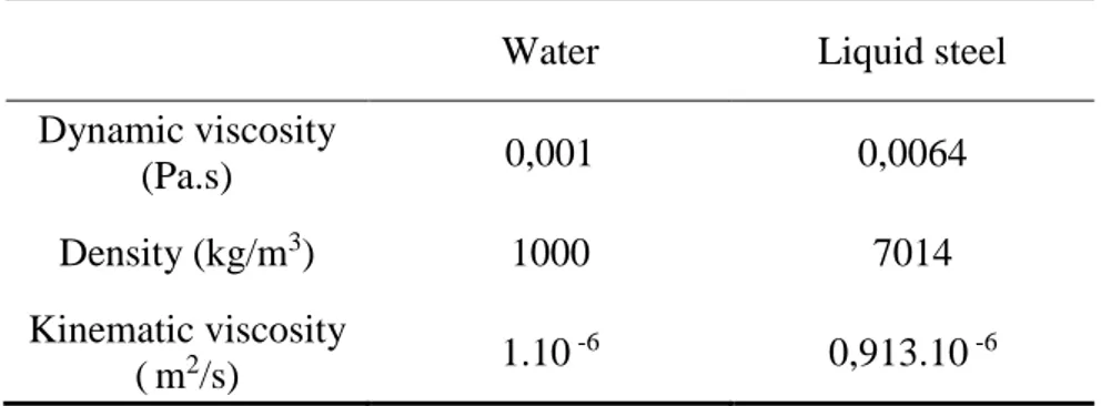
Reduced or full-scale water models have been used to assess crucial phenomena within the tundish. Water at 20ºC and liquid steel at 1600ºC have similar kinematic viscosities (dynamic viscosity/density), and hence make possible that important conclusions can be drawn from devices using water. Table 2.1 shows that kinematic viscosity of both fluids is of the same order of magnitude.

Table 2.1 – Physical properties of water at 20ºC and liquid steel at 1600ºC.

Water Liquid steel

Dynamic viscosity

(Pa.s) 0,001 0,0064

Density (kg/m3) 1000 7014

Kinematic viscosity

(m2/s) 1.10

-6 _0,913.10 -6

Source: Kemeny et al. (1981).

Anemometer (LDA) to determine the flow field into the tundish, thus forming the basis for a numerical model validation.

Through a wide range of design and operating parameters (tundish width, bath height, inlet-exit distance, inlet Froude number, tundish flow rate), Singh and Koria (1993) studied the molten steel fluid flow phenomena using a perspex glass water model. In this study, they found out that the proposed correlations were able to predict the fluid flow into the tundish very well, therefore, proper modifications could be proposed to existing devices and select optimal parameters to a new tundish.

2.3 Non-metallic inclusions

Non-metallic inclusions (mainly formed by oxides, sulfides, and nitrides), which arise from steel continuous casting process can be called as endogenous and exogenous. Endogenous inclusions are originated from deoxidation of products or precipitation of inclusions during cooling and solidification of steel. On the other hand, exogenous inclusions are formed through chemical reaction (reoxidation) and mechanical interaction among liquid steel, slag layer entrainment and lining refractory erosion (Zhang and Thomas, 2003).

In the steel continuous casting process, the level of steel cleanliness depends on the desired end products. Therefore, a maximum inclusion size is acceptable for specific steel products provided that this will not affect their final application. The maximum inclusion size for some steel products is shown in Table 2.2 (Zhang and Thomas, 2003).

Table 2.2 – Steel cleanliness requirements for maximum inclusion size.

Steel Product

Maximum inclusion size

 

Automotive industry 100

Pipelines 100

Wires 20

Ball bearings 15

Tire cords 10

Non-metallic inclusions do not pose any trouble for steel cleanliness if they stay as small as 1 m (Ishii et al., 2001). However, owing to intrinsic mechanisms of collision and

coagulation, they can become larger, and consequently may cause severe damages to the final product.

Amongst the several aspects that present vital influence over the mechanical behavior of steel, the size distribution is intrinsically important since larger inclusions are the most harmful to mechanical properties. As stated by Zhang and Thomas (2003), inclusions may reduce ductility, fracture toughness, corrosion resistance, hydrogen resistance to induced cracks, among others.

As non-metallic inclusion density has about half value of liquid steel density, they can be removed at the slag cover when they reach it by flotation mechanism. Therefore, the requirements for steel cleanliness can be satisfied. To achieve this, inclusions must stay into the tundish as much as possible in order to have enough time for them to float out. Therefore, steel makers have been making use of flow control devices to change the flow pattern into the tundish, to promote inclusion flotation, and to remove them by the slag layer.

2.4 Flow control modifiers

Figure 2.2 – Flow control modifiers (dams and weirs).

Source: Kemeny et al. (1981).

The weir can be thought of as a partial wall extending from the surface of molten steel to a certain level above the tundish bottom; on the other hand, the dam can be defined as a partial wall extending from the tundish bottom to a level below the slag cover.

According to Sahai and Ahuja (1986) the weir can guarantee low intensity of turbulence at slag slayer; however, it cannot eliminate short circuiting in a given tundish. Unlike the weir, dam can eliminate short circuiting completely, and besides this it has some others desired features such as the creation of surface directed flows, the increase in the mean residence time, and the trap of higher turbulent velocity values at the inlet region.

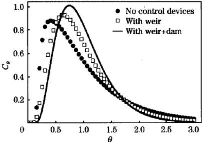
In the work of Bensouici et al. (2009), the position of flow control devices (dams and weirs) into the tundish was studied. It was concluded that these devices can promote floatation of non-metallic inclusions due to the above explanation. Some of their results are illustrated in Fig. 2.3.

Figure 2.3 – Typical RTD (Residence Time Distribution) curves for different tundish configurations.

Kemeny et al. (1981) performed experimental analysis into tundishes with no flow modifiers and also tested two different configurations, namely, one with dam only and another with dam and weir acting as flow modifiers. The authors evaluated the best location for the flow control devices through the analysis of characteristic times provided by RTD curves. A better tundish performance was found when the flow modifiers were inserted.

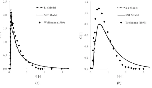
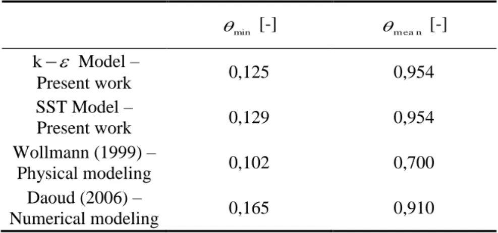
Wollmann (1999) tested four different types of flow modifiers in a physical analysis of a T-delta-shaped tundish, and he concluded that even with the simplest configuration of flow control device (using just one dam), an increase in mean residence time and elimination of short-circuiting could be observed.

Finally, it is worth noting that, in most of the times, the desired end results are made possible by making use of a combination of the aforementioned flow control devices, then, promoting higher rates of inclusion removal for a given tundish, and therefore to make the steel cleaner.

2.5 Thermal analysis applied to tundish modeling

Many studies have been carried out under isothermal conditions. However, non-isothermal fluid flow should be taken into account when actual tundishes are modeled, since temperature variation occurs from the inlet to the outlet of stream by heat losses to the atmosphere through walls and slag layer surface.

According to Sheng and Jonsson (1999), inside the tundish owing to low average flow velocity and high superheated temperature, there is a thermal buoyancy force that cannot be neglected and consequently, a thermal stratification will always exists inside the tundish.

As turbulence is decreased from inlet to the bulk fluid region, buoyant forces become predominant and hence natural convection plays an important role in the floatation of non-metallic inclusions in these regions (Ray, 2009). The non-isothermal behavior of molten steel into the tundish may cause significant changes in the mean residence time, temperature distribution, and inclusion movements (Sheng and Jonsson, 1999). Therefore, final products can be directly influenced by the non-isothermal field into the tundishes.

Figure 2.4 – Temperature contour on longitudinal plane.

Source: De Kock (2005).

In addition, in accordance with the above-mentioned study, Ray (2009) stressed out that in most of the studies in the literature, the temperature difference between the ladle shroud and the tundish outlet assumes values in the range of 15ºC to 25ºC.

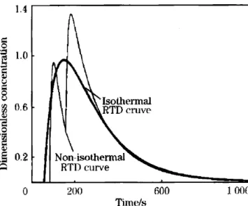
Alizadeh et al. (2008) carried out a steady state water modeling analysis under non-isothermal conditions in a twin-slab-strand continuous casting tundish. Their results showed that RTD curves were completely different under isothermal and non-isothermal conditions as can be seen in Fig. 2.5. Also, they related this divergence due to the presence of mixed convection phenomena in the non-isothermal tundish.

Figure 2.5 – Comparison between isothermal and non-isothermal RTD curves.

The present study considered the heat losses through the slag layer and walls only by radiation and convection heat transfer. The main mechanism of heat losses to the surroundings is found to be the radiation heat flux, since the latter mechanism is directly proportional to the fourth power of liquid steel temperature, while the convection heat losses are proportional to only the first power of molten steel temperature (Joo et al., 1993; Incropera and DeWitt, 1990). The summation of the aforementioned heat losses (energy/(area*time)) to the surroundings can be obtained by the following expression:









''

q h TT_  T T_ , (2.1)

where q'' denotes the total rate of energy per unity of superficial area of the tundish, h is the heat transfer coefficient by convection, T is the wall temperature (slag layer or tundish walls),



T is the room temperature,  is the Stefan-Boltzmann constant (5.67 x 10-8 _W/m2_.K4_{), and} 

is the material emissivity.

Generally, tundishes without any flow modifiers lose a significant amount of heat through their boundaries and hence the spatial temperature becomes nonuniformly. When adding some kind of flow control, the heat loss is reduced and then the temperature field must be more uniform (Szekely and Ilegbusi, 1989).

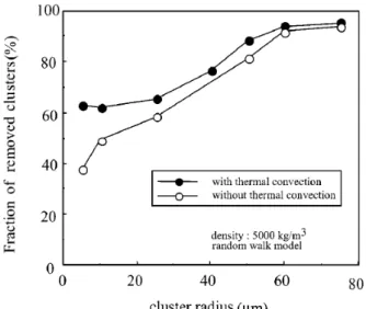
Miki and Thomas (1999) developed mathematical models to predict the removal of non-metallic inclusions from liquid steel in a continuous casting tundish (Al2O3 to be more

Figure 2.6 – Inclusion removal for isothermal and non-isothermal models.

Source: Miki and Thomas (1999).

Raghavendra et al. (2013) also studied the influence of thermally induced flows for inclusion flotation. The well-known open source CFD code, OpenFOAM, was used for modeling inclusion path in a four-strand asymmetric billet caster tundish. They obtained different fractions of removed particles when comparing isothermal and non-isothermal cases. However, different from the work of Miki and Thomas (1999), flows with buoyancy forces showed lesser separation efficiency for small particles at slag layer. The two works presented agreement with each other when large inclusion removal was considered.

2.6 Numerical methods applied to tundish modeling

Solving the Navier-Stokes equations analytically is only possible for a few simplified problems such as the fully developed Couette flow. When one deals with real flows, numerical methods must be used. Basically, by using a numerical approach the set of partial differential equations are transformed into a set of algebraic approximated equations.

One knows that any numerical procedure that obtain their approximate equations through a material balance is a finite-volume method. Thus, there are different types of the aforementioned method. One of them is the Element-based Finite-Volume Method (EbFVM), denomination suggested by Maliska (2004).

sub-elements according to the number of nodes of each element. In general, each sub-element is called sub-control volume because the conservation equations are integrated in time and space for each sub-element. After the integration process, the equation of each control-volume is assembled visiting all sub-control volumes that share the same node. Due to its conservative aspect, conservation of properties is guaranteed at each finite control volume.

Ansys CFX deals with three-dimensional meshes; the mesh can be composed of either hexahedral, tetrahedral, prism, and pyramid elements, or a combination of these elements. Nonetheless, for the sake of simplicity, a two-dimensional mesh, which is constructed with triangle and quadrilateral elements is described in Fig. 2.7. In this Figure, the blue numbers represent the elements, the sub-control volumes are represented by the SVC_i and, the control

volume related to the vertex 5 is described by green area. In general, hybrid meshes (combination of different elements) are used to better capture the physical phenomena of the problem to be solved. This approach has been successfully applied in several fields, see for instance, Marcondes and Sepehrnoori (2010), Pimenta (2014), and Filippini et al. (2014).

Figure 2.7 – Unstructured mesh and control-volume.

Source: Fernandes (2014).

During the process, all variables and material properties are stored at the nodes. Joining the edge centers and element centers, a control volume is then constructed around each node. This is called median dual method (Ansys CFX, 2011), and gives rise to a cell-vertex approach.

Diffusion terms do not pose numerical instabilities when interpolation schemes are applied to interpolate physical properties from the nodes to the integration points (owing to their elliptic behavior); on the other hand, care should be taken when advective terms are involved. The use of non-exact interpolation functions gives rise to truncation errors. When these errors are associated with advective terms, numerical oscillation and numerical diffusion errors are yielded (Maliska, 2004).

To achieve physically realistic numerical results, interpolation schemes must possess fundamental properties. The most relevant ones are conservativeness, boundedness and transportiveness (Versteeg and Malalasekera, 2007).

2.7 Turbulence Models

When fluid flows are controlled by viscous diffusion of vorticity and momentum, they are called laminar flows, and the Reynolds number is in general small. As Reynolds number increases, the inertia terms overcome the viscous stresses, and consequently rapid velocity and pressure fluctuation appear in the fluid flow and the motion becomes inherently three-dimensional and unstable, which can be described as a turbulent flow (Wilcox, 2006).

Turbulent eddies, which can be thought of as a local swirling motion where the vorticity can often be very intense, appear in a wide range of sizes and permit mixing and effective turbulent stresses to come up. Turbulence is mainly dominated by larger eddies as highlighted by Wilcox (2006).

The unsteady Navier-Stokes equations are capable of computing the smallest length and time scales of turbulence. However, these calculations are not feasible in terms of computing resources, since temporal and spatial grids need to be sufficiently fine in order to resolve all turbulent scales. Besides, for practical engineering applications the assessment of smaller eddies when compared to the larger eddies are not important.

is not practicable for modeling actual 3D turbulent flow in tundishes (Omranian, 2007; Chattopadhyay et al., 2010).

By using the LES approach, the large scale quantities are fully solved while the small scales are modeled. A spatial filtering approach separates the resolved turbulent scales from the modeled ones. LES is less accurate than DNS, however, it is numerically more economic (Argyropoulos and Markatos, 2015). Gardin et al. (2002) used an RNG subgrid-scale LES model, which is available in the commercial software FLUENT, to perform numerical analysis for a given tundish. Even though the agreement with experimental results were not good and convergence time took so long, they concluded that through the adjustment of some constants, the LES model can work both for the jet spreading and the wall jet predictions.

RANS is based on averaging the equations of motion resulting in a set of partial differential equations. In spite of having some limitations, due to the averaging process, to date the RANS models are still the first choice when numerical tundish modeling is required.

When averaging mass and momentum equations, additional terms appear and therefore this form a non-closed set of equations. These new terms are called Reynolds stresses, and as a result of this further information is necessary to balance the equations and the unknowns. Turbulence models are responsible for computing Reynolds stresses, and then close the system of mean flow equations in order to make the solution possible.

Commonly, RANS turbulence models are grouped into classes based on the number of additional transport equations that need to be solved together with the mean flow equations (Versteeg and Malalasekera, 2007). Table 2.3 presents the number of additional variables for each turbulence model.

Table 2.3 – Turbulence models.

No. of extra transport equations Turbulence Model

Zero Mixing Length Model

One Sparlat-Allmaras Model

Two k-ε Model

k-ω Model Algebraic Stress Model

Seven Reynolds Stress Model

The fluid flow into the tundish is promoted by the nozzle that is placed at the exit of the ladle. At the inlet region (and also at outlet) of the tundish the flow regime is mostly turbulent, while far from the inlet (bulk region), turbulence decreases progressively, and hence inclusions can be removed (Gardin et al., 2002).

Accuracy is most required at inlet region in order to analyze correctly both the spreading rates of the jet and impinging wall boundary layer, consequently a local refined grid in conjunction with a good turbulence model need to be used (Gardin et al., 2002).

It is observed that two-equation models are the first ones preferred by industry. Also, two-equations eddy viscosity models are still preferable for CFD calculations, with the standard k model (Launder and Sharma, 1974) and k model (Wilcox, 1988) being the most widely used. Researchers have applied k model exhaustively for the tundish modeling and this model is currently considered to be well tested. Also, good agreements with experimental studies have been achieved with the application of this model.

The tundish metallurgy area has been following this tendency since k model has been massively employed over the years by many authors to account for turbulence quantities (Yeh et al., 1994; Daoud, 2006; Tiang-peng et al, 2012; Alves, 2014).

Despite of being exhaustively used, according to Ilegbusi (1994), k turbulence model has some tendency to overestimate mixing in regions, where turbulent and laminar regimes are present; such situation often occurs in vessels like tundishes. Accordingly, each region (turbulent and laminar) of the tundish domain must be properly modeled by making use of a suitable turbulence model.

In order to figure out how turbulent quantities behave inside tundishes, several authors have performed studies analyzing different types of turbulence models. Jha and Dash (2004) studied the numerical prediction of tracer concentration at tundish outlet with six different turbulence models, namely, the standard k, the k RNG, the low-Reynolds number Lam-Bremhorst model, the Kim high-Reynolds number model (CK), the Chen-Kim low-Reynolds number model (CKL), and the simplest constant effective viscosity model (CEV). Gardin et al. (2002) used the k model, three types of low-Reynolds number k

model variants, and the RNG sub-grid scale model (LES-model) to take into account the viscous damping away from the walls. The analysis showed that both the k model and the LES model did not produce good agreement with experimental measurements whereas the k

More advanced turbulence models have been proposed, one of them is the Shear Stress Transport (SST) model, which combines the advantages of both k and k model. SST activates k model in the near-wall region and the k model for the remainder of the flow (Menter et al., 2003). Kruger (2010) suggested the use of SST model due to the above explanations, and indeed good results were achieved by him.

Taking into account the above explanations, the k turbulence model was employed in the present study for some simulations in order to test its efficiency in modeling the fluid flow phenomena in tundishes. However, most simulations, including fluid flow, heat transfer, and Lagrangian analysis were made by making use of the SST turbulence model.

2.8 RTD (Residence Time Distribution) analysis

One way to assess information about fluid flow in a tundish, either numerically or experimentally, is perform a stimulus-response experiment through the injection of a tracer (non-reactive tracers are widely used) in the incoming flow and monitoring its concentration at exit. By plotting this concentration against time, one obtains the so-called Residence Time Distribution (RTD) curve or C-curve. Residence time can be defined as the time that a single fluid element spends within any vessel. This distribution curve is originated from the fact that some fluid element spend more time within the tundish than others (Mazumdar and Guthrie, 1999).

Figure 2.8 – Combined model.

Source: Sahai and Emi (1996).

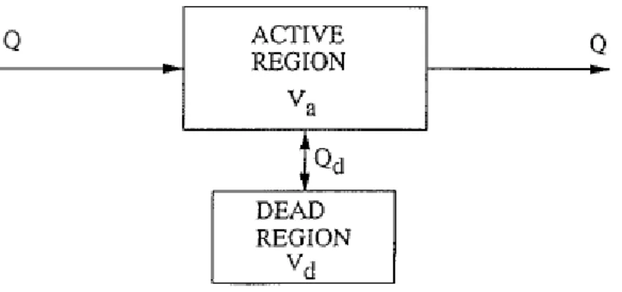
In addition, the combined model can be grouped into an active region (a combination of plug and well mixed volumes) and a dead region as can be seen in Fig. 2.9.

Figure 2.9 – Fluid flow crossing the active and dead regions in a combined model.

Source: Sahai and Emi (1996).

Having described the characteristic volumes, one notes that some important characteristic times are also worth to mention. They are defined as follows:

• Theoretical residence time, t

The theoretical residence time depends only on the geometric and operational parameters and it is obtained dividing the tundish volume, V, by the volumetric flow rate, q .

V

t ,

q

 (2.2)

• Minimum residence time, t_min

The minimum residence time can be defined as the time when the first fluid element leaves the tundish. In a tracer pulse experiment, it is represented by the first detected concentration of the tracer at the exit.

• Mean residence time

The mean residence time stands for the mean time spent by all fluid elements into a given tundish.

• Maximum residence time, t_peak

The maximum residence time represents the time when the maximum quantity of fluid elements leave a given tundish.

In order to avoid some external influence, such as amount of tracer mass, tundish volume, inlet volumetric flow rate, as well as to compare different kinds of tundishes, the C-curve must be put in a dimensionless form.

According to Levenspiel (1998), each dimensionless residence time, , is obtained

dividing each instant of time, t_i, by the theoretical residence time, t, therefore, we have:

i t

, t



 (2.3)

min min t , t 

 (2.4)

peak peak t , t 

where _min and _peak stand for the dimensionless form of the minimum and maximum residence time, respectively.

To normalize the tracer concentration, C_i, collected at the outlet of the tundish at

each instant of time, the tracer mass, m_t, as well as the tundish volume, V, are related by the

following expression, resulting in a dimensionless form of the concentration, C (Levenspiel, 1998): i t C C , m V

 (2.6)

The dimensionless mean residence time is calculated through the Residence Time Distribution (RTD) curve. If the concentration at the exit is measured at equal time intervals,

the dimensionless mean residence time,  , is calculated as follows:

0 0     





The dead volume fraction can be calculated through the following expression:

1 a D C Q V ,

V   Q 

(2.8)

In the above expression, Q_a represents the volumetric flow rate through the active

region and Q the total volumetric flow rate through the tundish. The term, Qa

Q , is expressed by

the area under the RTD curve from  0 to  2.

2 0 a i Q C ,

Q 



(2.9)

2 0 2 0 i i C i C , C       





Considering that the minimum residence time, _min, and maximum residence time,

peak

 show different values, the fraction of plug volume is calculated as (Sahai and Ahuja, 1986):

2

min peak P

V   , (2.11)

Finally, all volume fractions must be equal to unit, then the well mixed volume fraction is expressed by:

1

M P D

V   V V . (2.12)

Some regions of a given tundish with and without flow modifiers are showed in Fig. 2.10. This figure emphasizes the presence of dead volume in tundish corners and the leeward side of the flow control devices (dams and weirs).

Figure 2.10 – Tundish volume regions.

Source: Shade et al. (1996).

Based on the characteristic times and volumes, the behavior of the fluid flow as well as the probability for removing non-metallic inclusions by the slag layer may be available, which can be used to propose modifications to the tundish configuration in order to improve the steel quality.

Sahai and Ahuja (1986) pointed out that to achieve maximum inclusion separation ratio in a continuous casting tundish, the following characteristics should be ensured:

• Minimum spread of residence times; • Minimum dead volume;

• Large ratio of plug to dead volume and relatively large ratio of plug to well-mixed volume;

• Flow directed to the top surface; • Quiescent slag layer;

• Contained regions of mixing.

3 METHODOLOGY

The steps involved in modeling the steel continuous casting tundish using the commercial software Ansys CFX are illustrated in Fig. 3.1.

Figure 3.1 – Work methodology.

First, the geometry as well as the mesh were created using the Ansys ICEM CFD software. In the pre-processing step in Ansys CFX, the computational domain, initial and boundary conditions, working fluids (steel and water), material properties, time-steps, interpolation function, number and diameter of particles injected at inlet, steady state or transient analysis, and so on, were all defined.

The mass, momentum, energy, turbulence, tracer convection-diffusion, and particle tracking equations are solved along with initial and boundary conditions with a coupled solver using the Element-based Finite-Volume Method (EbFVM).

4 MATHEMATICAL FORMULATION

The governing equations of mass, momentum, and energy were applied to compute the flow field and heat transfer within the tundish. The turbulence models have been used for calculating turbulence quantities without using Direct Numerical Simulation (DNS). For calculating the tracer concentration at the outlet tundish region a convective-diffusion transport equation was applied. Finally, in order to obtain the fraction of particles removed at slag cover, a Lagrangian tracking equation was employed.

4.1 Mass and momentum equations

In turbulent flows the instantaneous quantities, such as velocity and pressure are separated into mean and fluctuating parts, which gives rise to the well-known Reynolds Averaged Navier-Stokes (RANS) approach.

After averaging continuity and momentum equations and using the Boussinesq eddy-viscosity approximation to relate the Reynolds stresses to the strain rate of the mean motion, we obtain

 

j U , t x  _  _  _   (4.1)

 









i i j eff ref ref

j i j j i

U U p

U U U g T T ,

t  x  x x  x x  

(4.2)

where  is fluid density, U_j are velocity components, p is pressure, _ref is a reference density,

g is gravitational acceleration, T is temperature, T_ref is a reference temperature, and _eff represents the effective viscosity accounting for turbulence, which is defined by

eff t,



 

For the momentum equation in the y-direction, the buoyant term is modeled by the Boussinesq model. In this model, it is assumed that density is constant, except for the buoyant term that is modeled by





 ref   ref TTref ,

    (4.4)

in which



1     _{ }

  p ref

, T 

 _ (4.5)

This approximation is acceptable since the variation of the density of the liquid steel in actual processes due to the temperature difference is quite small.

4.2 Turbulence models

For modeling turbulence quantities, the two-equation k model as well as the SST model were used, thereby two additional variables were introduced into the system of equations.

4.2.1 kturbulence model

The k model assumes that the turbulence viscosity is related to the turbulence kinetic energy k and the turbulence eddy dissipation  by the following relation:

2

t

k

C_ ,





_

where C_ is a constant.

 

j k

j k j

k

k U k P ,

t x x

   _    _  _{ }  _{ }     _  _ (4.7)

 





eff

j k

j j

U C P C ,

t x _ x k  

      _    _  _{ }  _{ }     _  _ (4.8)

where C_1, C_2, _k, and _ are constants taken from Launder and Spalding (1974). P_k is the turbulence production owing to viscous forces and it is given by

      _ _{ }  _ _   j i i k t

j j i

U

U U

P .

x x x

(4.9)

4.2.2 SST turbulence model

The two-equation SST turbulence model consists of a blending between the k

turbulence model near the wall and the k turbulence model far away from the walls. This interchange is made through a blending function F₁, which assumes a value of one near the

solid surface and zero in the outer region of the flow (Menter et al., 2003). To obtain the transport equations for the turbulent kinetic energy k and the turbulence frequency



model is multiplied by F₁ and a modified form of the k model is multiplied by 1F₁

(Ansys CFX, 2011), resulting in the following equations:

 

 

3

' t

j k

j j k j

k

k U k P k ,

t x x x

    _       _  _  _  _{ }       _{ } _ (4.10)

 









3 3 2 3 3 1 1 2 t j

j j j j j

k

k

U F

t x x x x x

where _k3,



, ₃ are constants taken from Menter et al. (2003). The blending function F1 is based on the distance to the nearest wall y as well as the flow variables, and it

is calculated as follows:

 

1 1

F tanh arg , (4.12)

with:

1 2 2

2

500 4

'

k

k k

arg min max , , ,

y y CD_{ } y

           _ _ _ _     (4.13)

where  is the kinematic viscosity (dynamic viscosity/density) and:

10 3

1

2 1 0 10

k

j j

k

CD max , . x .

x x    _{ }   _{ }   _{  } _   (4.14)

Therefore, the turbulent viscosity is calculated from:





t

a k ,

max a ,SF

  _ (4.15)

where

t

t .





_

Sstands for an invariant measure of the strain rate and a is a constant taken from ₁

Menter et al. (2003). The blending function F is given by: ₂

 

2 2

F tanh arg , (4.17)

2 2

2 500

'

k

arg max , .

y y        _{ }   (4.18)

4.3 Thermal energy equation

Thermal energy equation is derived from the first law of thermodynamics. By assuming that the conductive heat fluxes are expressed by the Fourier’s law and neglecting the radiative and viscous dissipation effects for an incompressible flow, the final form of the energy equation can be written as:

 

 

j j j

T

h U h K ,

t  x  x x

 

 _  _  _  _

 

   _  _

(4.19)

where h is the enthalpy and K_eff is the effective thermal conductivity, which we may define as:

p t eff

t C

K K ,

Pr 

  (4.20)

where K is the thermal conductivity, C is the specific heat at constant pressure, and _p Pr_t is the

turbulent Prandtl number.

4.4 Tracer convection-diffusion equation

To obtain the RTD curve, it is necessary to solve an additional conservation equation. Therefore, the tracer (which is considered to be a passive scalar) distribution all over the domain is solved through the following advection-diffusion equation:

 





j j j

C

C U C D ,

t  x  x x

 

 _  _  _  _

 

   _  _

(4.21)

where C is the tracer concentration and D_eff is the effective kinematic diffusivity, which is

t eff

c

D D ,

S





  (4.22)

where D is the kinematic diffusivity and S_c is the turbulent Schmidt number.

4.5 Particle tracking equation

The Lagrangian analysis is used when distinguishable mass elements are easy to follow. This analysis can be applied to describe a whole flow field (considering that the flow field is composed by a large number of particles). However, following each particle by itself might be a cumbersome process. Nevertheless, the Lagrangian modeling can be used to the present work as the non-metallic inclusions are treated as a small number of particulates immersed in the fluid domain. In this formulation, the particle tracking is performed through a force balance, which are acting on each of them.

Lagrangian particle tracking method solves a transport equation for each non-metallic inclusion in order to describe their paths. The present work is based on one-way coupling interaction between liquid and solid phases, i.e., the inclusion trajectories, which are calculated through the previously calculated flow field, are influenced by the flow field and the opposite do not occur.

Applying a force balance on each particle and accounting for only their drag and buoyancy forces relative to the molten steel, since they represent the main forces on the particle (Yuan and Thomas, 2005), the inclusion path can be described as follows:









2 3

1 1

8 6

p

p p D p p p p

dU

m d C U U U U d g ,

dt 

 



 

(4.23)

where

m

the diameter d_p and the density of the particle _p to perform the analysis.





24

max 1 0 15 . 0 44

D

C . Re , . ,

Re

 

 _  _

 

(4.24)

The particle Reynolds number is defined as follows:

p p U U d

Re  .





 (4.25)

The second term on the right-hand side in Eq. (4.23) accounts for the influence of buoyancy forces on the fluid due to gravitational acceleration.

In order to simulate the random effect of turbulent eddies over the inclusion trajectories, a Random Walk Model (RWM) was used. In this model, the instantaneous velocity fluctuations depend on the local level of turbulent kinetic energy and a random number distributed between -1 and 1. Further details on this model can be found elsewhere (Crowe et al., 1998; Vargas-Zamora et al., 2003).

Miki and Thomas (1999) evaluated the influence of the Random Walk Model on trajectories of inclusions. Fig. 4.1 presents the fraction of removed particles with and without the Random Walk Model for different particle densities.

Figure 4.1 – Inclusion removal with and without the Random Walk model.

Source: Miki and Thomas (1999).

According to Javurek (2002), if we decrease the diameter of the particle and the rising velocity towards a zero value, the particle tracking equation approaches the RTD curve model.

4.6 Initial and Boundary conditions

The present section describes all details related to initial and boundary conditions used in case studies I, II, and III. For the sake of simplicity, details concerning the validation cases were omitted. Thus, the boundary conditions, which were used for solving the steady-state analysis, are steady-stated as follows:

• Inlet region:

At inlet, a prescribed value for normal velocity (3,57 m/s) was calculated based on the casting speed and the transverse section of a common billet produced at a local steelmaker company. These data are shown in Tables 5.2 and 5.3, which were presented in the previous section.

A prescribed value for temperature (1823K) was based upon actual operation temperature as it is also shown in Table 5.3. The turbulence intensity was set to 5% in order to account for turbulence quantities. For Lagrangian analysis, particles were injected uniformly and assuming the same value of the fluid velocity.

• Outlet region:

At the exit nozzle, a prescribed value of 0 Pa was set for pressure. • Walls:

At tundish walls, including dams and weirs, no-slip conditions were prescribed. An automatic near wall treatment was applied for SST model and a scalable wall function for k

model (Ansys CFX, 2011). For the non-isothermal analysis, a prescribed flux of 9000 W/m2 was set for all tundish walls, except for dams and weirs, which were considered to be adiabatic (De Kock, 2005). When considering Lagrangian analysis, a restitution coefficient equal to 1 was applied; Therefore, all collisions were considered to be perfectly elastic.

• Free surface of steel bath:

At the slag cover, free-slip condition (zero shear stress) was applied. Furthermore, a prescribed flux of 18000 W/m2 was applied (De Kock, 2005). For Lagrangian analysis, a restitution coefficient equal to 0 was applied; Therefore, all particles that collided with the slag layer were captured.