660 Brazilian Journal of Physics, vol. 36, no. 3A, September, 2006
Critical Behavior of the Spin-
3/2
Blume-Capel Model on a
Random Two-Dimensional Lattice
F. W. S. Lima1 and J. A. Plascak2
1Departamento de F´ısica, Universidade Federal do Piau´ı , 57072-970, Teresina, PI, Brazil
2Departamento de F´ısica, Universidade Federal de Minas Gerais, C. P. 702, 30123-970, Belo Horizonte, MG, Brazil
Received on 9 November, 2005
We investigate the critical properties of the spin-3/2 Blume-Capel model in two dimensions on a random lattice with quenched connectivity disorder. The disordered system is simulated by applying the cluster hybrid Monte Carlo update algorithm and re-weighting techniques. We calculate the critical temperature as well as the critical point exponentsγ/ν,β/ν,α/ν, andν. We find that, contrary of what happens to the spin-1/2 case, this random system does not belong to the same universality class as the regular two-dimensional ferromagnetic model.
Keywords: Random lattices; Blume-Capel model; Hybrid Monte Carlo; Universality
I. INTRODUCTION
Experimental studies of the critical behavior of real mate-rials are often confronted with the influence of impurities and inhomogeneities [1]. For a proper interpretation of the mea-surements it is, therefore, important to develop a firm theoret-ical understanding of the effect of such random perturbations. In many situations the typical time scale of the thermal fluc-tuations in the idealized “pure” systems is clearly separated from the time scale of the impurity dynamics, such that to a very good approximation the impurities can be treated as quenched. The importance of the effect of quenched random disorder on the critical behavior of a physical system can be classified by the specific heat exponent of the pure system, αpure. The criterion due to Harris [2] asserts that forαpure>0 quenched random disorder is a relevant perturbation, leading to a different critical behavior than in the pure case (which is the case of the three-dimensional Ising model). In particular, one expects [3] in the disordered system thatν≥2/D, where νis the correlation length exponent andDis the dimension of the system. Assuming hyper-scaling to be valid, this implies α=2−Dν≤0. On the other hand for αpure<0 disorder is irrelevant (as is the case of the three-dimensional Heisen-berg model) and, in the marginal caseαpure=0, no prediction can be made. For the case of (non-critical) first-order phase transitions it is known that the influence of quenched random disorder can lead to a softening of the transition [4]. Recently, the predicted softening effect at first-order phase transitions has been confirmed for 3D q-state Potts models with q≥3 using Monte Carlo [5–7] and high temperature series expan-sion [8] techniques. The overall picture is even better in two dimensions (2D) where several models withαpure>0 [9–12] and the marginal (αpure=0) [13–17] have been investigated.
In this paper we study another type of quenched ran-dom disorder, namelyconnectivity disorder, a generic prop-erty of random lattices whose local coordination number varies randomly from site to site. Specifically, we consider 2D Poissonian random lattices of Voronoi-Delaunay type, and performed an extensive computer simulation study of a Blume-Capel model. We concentrated on the close vicinity
of the transition point and applied finite-size scaling (FSS) techniques to extract the exponents and the “renormalized charges”U2∗andU4∗. To achieve the desired accuracy of the data in reasonable computer time we applied the single-cluster hybrid algorithm [18] to update the spins and furthermore made extensively use of the re-weighting technique [19]. Pre-vious studies of connectivity disorder focusing mainly on 2D lattices have been realized by Monte Carlo simulations ofq -state Potts models on quenched random lattices of Voronoi-Delaunay type for q=2 [20–22], q =3 [23] and q =8 [24, 25]. In particular, it has been shown that forq=2 [20– 22] andq=3 [23] the critical exponents are the same as those for the model on a regular 2Dlattice. This is indeed a sur-prising result since the relevance criterion of the Delaunay tri-angulations reduces to the well known Harris criterion such that disorder of this type should be relevant for any model with positive specific heat exponent [26]. This means that for q=3, whereαpure>0, one would expect a different univer-sality class. On the other hand, for the present spin-3/2 model, whereαpure=0, we show that the exponents indeed change in the Voronoi-Delaunay lattice type, turning out the situation still more bizarre . In the next section we present the model and the simulation background. The results and conclusions are discussed in the last section.
II. MODEL AND SIMULATION
tessella-F. W. S. Lima and J. A. Plascak 661
tion.
We consider now the two-dimensional spin-3/2 Capel model on this Poissonian random lattice. The Blume-Capel Model is a generalization of the standard Ising model [28] and was originally proposed for spin-1 to account for first-order phase transition in magnetic systems [29, 30]. The Hamiltonian can be written as
H=−J
∑
<i,j>
SiSj+∆
∑
iS2i, (1)
where the first sum runs over all nearest-neighbor pairs of sites (points in the Voronoi construction) and the spin-3/2 variables Siassume values±3/2,±1/2. In eq. (1)Jis the exchange coupling and ∆is the single ion anisotropy parameter. The second sum is taken over theNspins on aD-dimensional lat-tice. The case whereS=1 has been extensively studied by several approximate techniques in two- and three-dimensions and its phase diagram is well established [29–35]. The case S>1 has also been investigated according to several proce-dures [36–42].
The simulations have been performed for∆=0, which is the simplest case, on different lattice sizes comprising a num-ber N =1000,2000,4000,8000, 16000 and 32000 of sites. For simplicity, the length of the system is defined here in terms of the size of a regular latticeL=N1/2. For each system size quenched averages over the connectivity disorder are approxi-mated by averaging overR=100 (N=1000 to 4000),R=50 (N=8000) andR=25 (N=16000 and 32000) independent realizations. For each simulation we have started with a uni-form configuration of spins (the results are however indepen-dent of the initial configuration). We ran 2.52×10⁶ Monte Carlo steps (MCS) per spin with 1.2×10⁵configurations dis-carded for thermalization using the “perfect” random-number generator [43]. We have employed the hybrid algorithm [18] where we includednWolff clusters (heren=5) intercalated by one Metropolis single-spin flip sweep. This algorithm has been shown to be quite effective for spin-3/2 models [18]. For every 12th MCS, the energy per spin,e=E/N, and magneti-zation per spin,m=∑iSi/N, were measured and recorded in a time series file.
From the series of the energy measurements we can com-pute, by re-weighting over a controllable temperature interval ∆T, the average energy and specific heat
e(K) = [<E>]av/N, (2)
C(K) =K2N[<e2>−<e>2]av, (3) whereK=J/kBT, withJ=1, andkBis the Boltzmann con-stant. In the above equations < ... >stands for thermody-namic averages and[...]av for averages over the different re-alizations. Similarly, we can derive from the magnetization measurements the average magnetization, the susceptibility, and the magnetic cumulants,
m(K) = [<|m|>]av, (4)
χ(K) =KN[<m2>−<|m|>2]av, (5)
U2(K) = [1−
<m2>
3<|m|>2]av, (6)
U4(K) = [1−
<m4>
3<|m|>2]av. (7) Further useful quantities involving both the energy and mag-netization are their derivatives
d[<|m|>]av
dK = [<|m|E>−<|m|><E>]av, (8)
dln[<|m|>]av
dK = [
<|m|E>
<|m|> −<E>]av, (9)
dln[<|m2|>]av
dK = [
<|m2|E>
<|m2|> −<E>]av. (10) In the infinite-volume limit these quantities exhibit singulari-ties at the transition point. In finite systems the singularisingulari-ties are smeared out and scale in the critical region according to
C=Creg+Lα/νfC(x)[1+...], (11)
[<|m|>]av=L−β/νfm(x)[1+...], (12)
χ=Lγ/νfχ(x)[1+...], (13)
dln[<|m|p>]av
dK =L
1/νfp(x)[1+...], (14) whereCreg is a regular background term, ν,α,β, and γare the usual critical exponents, and fi(x)are FSS functions with x= (K−Kc)L1/νbeing the scaling variable, and the brackets [1+...]indicate corrections-to-scaling terms. We calculated the error bars from the fluctuations among the different re-alizations. Note that these errors contain both, the average thermodynamic error for a given realization and the theoret-ical variance for infinitely accurate thermodynamic averages which are caused by the variation of the quenched, random geometry of the lattices.
III. RESULTS AND CONCLUSION
662 Brazilian Journal of Physics, vol. 36, no. 3A, September, 2006
0.180 0.182 0.184 0.186 0.188 0.190
K
0.3 0.4 0.5 0.6 0.7
U4 1000 32000
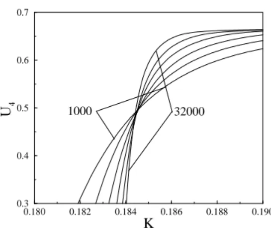
FIG. 1: Fourth-order Binder cumulant as a function ofK for sev-eral values of the system sizeN=1000,2000,4000,8000,16000 and 32000.
3.2 3.8 4.2 4.8 5.2
Ln L 5.2
5.8 6.2 6.8 7.2 7.8
Ln(d(ln<|m|
p >)/dk)
max
p=1 p=2
FIG. 2: Log-log plot of the maxima of the logarithmic derivative
dln[<|m|p>]
dK versus the lattice sizeL=N1/2 for p=1 (circle) and p=2 (square). The solid lines are the best linear fits.
In order to estimate the critical temperature we calculate the second and fourth-order Binder cumulants given by eqs. (7) and (8), respectively. It is well known that these quantities are independent of the system size and should intercept at the critical temperature [44]. In Fig. 1 the fourth-order Binder cumulant is shown as a function of theK for several values ofN. Taking the largest lattices we have Kc=0.1844(1).
To estimateU4∗we note that it varies little at Kc so we have
U4∗=0.482(6). From the second-order cumulant we similarly getKc=0.1845(1)andU2∗=0.579(8). One can see that the agreement of the critical temperature is quite good andU4∗is definitely far from the universal valueU4∗∼0.61 for the same model on the regular 2Dlattice.
The correlation length exponent can be estimated from the derivatives given by eq. (15). Fig. 2 shows the maxima of the logarithm derivatives as a function of the logarithm of the lattice sizeLforp=1 andp=2. From the linear fitting one getsν=0.85(2)(p=1) andν=0.917(8)(p=2), which is again different from the regular lattice exponentν=1.
In order to go further in our analysis we also computed
3.2 3.8 4.2 4.8 5.2
Ln L
−2.2 −2.0 −1.8 −1.6 −1.4 −1.2
Ln(<|m|>)
inf
FIG. 3: Plot of the logarithm of the modulus of the magnetization at the inflection point as a function of the logarithm ofL=N1/2. The solid line is the best linear fit.
3.25 3.75 4.25 4.75 5.25
Ln L
1.00 1.50 2.00 2.50 3.00 3.50 4.00 4.50
Ln
χmax
FIG. 4: Log-log plot of the susceptibility maximaχmaxas a function
of the logarithm ofL=N1/2. The solid line is the best linear fit.
the modulus of the magnetization at the inflection point and the maximum of the magnetic susceptibility. The logarithm of these quantities as a function of the logarithm of L are presented in Figs. 3 and 4, respectively. A linear fit of these data givesβ/ν=0.331(9)from the magnetization and γ/ν=1.467(9)from the susceptibility which should be com-pared toβ/ν=0.125 andγ/ν=1.75 obtained for a regular 2Dlattice.
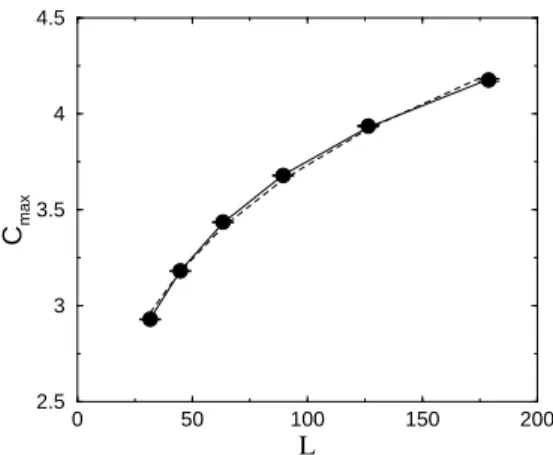
The specific heat can also be analysed in this case but, as it happens in other models [21, 23], we cannot find a clear unambiguous support for a definite scaling. Fig. 5 shows the maximum of the specific heat Cmax as a function of L.
Least-squares fits to a logarithmic AnsatzCmax=B0+B1lnL giveB0=0.44(6),B1=0.72(1)and is shown by the full line in Fig. 5. The dashed line in this figure corresponds to a pure power-law Ansatz,Cmax=cLα/νwithc=1.475(5)and
α/ν=0.202(5). From these results one can slightly see a better agreement with the logarithmic Ansatz.
F. W. S. Lima and J. A. Plascak 663
0 50 100 150 200
L
2.5 3 3.5 4 4.5
Cmax
FIG. 5: Specific heat maximaCmax as function ofL=N1/2. The solid line is the best fit to anα∼0 (Log) Ansatz and the dashed line to a power law Ansatz.
done Janke and Weigel on the Harris-Luck criterion for ran-dom lattices [26], another open question to be answered in more general terms.
[1] D. P. Belanger, Braz. J. Phys.30, 682 (2000). [2] A. B. Harris, J. Phys. C7, 1671, (1974).
[3] J. Chayes, L. Chayes, D. S. Fisher, and T. Soencer, Phys. Rev. Lett.57, 299 (1986).
[4] Y. Imry, M. Wortis, Phys. Rev. B19, 3581 (1979).
[5] H. G. Ballestros, L. A. Fernandez, V. Martin-Mayor, A. Munoz Sudupe, G. Parisi, and J. J. Ruiz-Lorenzo, Phys. Rev. B 61, 3215 (2000).
[6] C. Chatelain, B. Berche, W. Janke, and P. E. Berche, Phys. Rev.
E 64, 036120(2001).
[7] C. Chatelain, P. E. Berche, B. Berche, and W. Janke, Nucl. Phys. B (Proc. Suppl.)106-107, 899 (2002).
[8] M. Hellmund and W. Janke, Nucl. Phys. B (Proc. Supl.) 106-1-7, 923 (2002).
[9] D. Matthews-Morgan, D. P. landau, and R. H. Swendsen, Phys. Rev. lett.53, 679 (1984).
[10] M. A. Novotony and D. P. Landau, J. Mag. Magn. Mater.15-18, 247 (1980).
[11] G. Jug and B. N. Shalaev, Phys. Rev. B54, 3442 (1996). [12] S. Wiseman and E. Domany, Phys. Rev. E51, 3074 (1995). [13] Vik. S. Dotsenko and VI. S. Dotsenko, Adv. Phys. 32, 129
(1983).
[14] A. Roder, J. Adler, and W. Janke, Phys. Rev. Lett.80, 4697 (1988).
[15] F. D. A. Aar˜ao Reis, S. L. A. de Queiroz, and R. R. dos Santos, Phys. Rev. B566013 (1997).
[16] P. H. L. Martins and J. A. Plascak, to be published. In this work the use of the probability distribution function is used to show that the universality class of the 2Ddiluted Ising model is in fact the same as that of the pure model.
[17] P. H. L. Martins and J. A. Plascak, Braz. J. Phys.34, 433 (2004). [18] J. A. Plascak, Alan M. Ferrenberg, and D. P. Landau, Phys. Rev.
E65,066702 (2002).
[19] A. M. Ferrenberg and R. H. Swendsen, Phys. Rev. Lett. 61, 2635 (1988).
[20] D. Spriu, M. Gross, P. E. L. Rakow, and J. F. Wheater, Nucl. Phys. B265[FS15], 92 (1986).
[21] W. Janke, M. Katoot, and R. Villanova, Phys. Lett B315, 412 (1993).
[22] F. W. S. Lima, J. E. Moreira, J. S. Andrade Jr., and U. M. S. Costa, Physica A283, 100 (2000).
[23] F. W. S. Lima, U. M. S. Costa, M. P. Almeida, and J. S. Andrade Jr. Eur. Phys. J. B17, 111 (2000).
[24] W. Janke and R. Villanova, Phys. Lett. A209, 179 (1995). [25] F. W. S. Lima, J. E. Moreira, J. S. Andrade Jr., and U. M. S.
Costa, Eur. Phys. J. B13, 107 (2000).
[26] W. Janke and M. Weigel, Phys. Rev. E69, 144208 (2004). [27] N. H. Christ, R. Friedberg, and T. D. Lee, Nucl. Phys. B202,
89 (1982); B210[FS6] 310, 337 (1982). [28] S. Kobe, Braz. J. Phys.30, 649 (2000).
[29] M. Blume, Phys. Rev.141, 517 (1966); H. W. Capel, Physica (Amsterdam)32, 966 (1966).
[30] M. Blume, V. J. Emery, and R. B. Griffths, Phys. Rev. A4, 1071 (1971).
[31] D. M. Saul, M. Wortis, and D. Staufer, Phys. Rev. B9, 4964 (1974).
[32] A. K. Jain and D. P. Landau, Phys. Rev. B22, 445 (1980). [33] O. F. de Alcantara Bonfim, Physica A130, 367 (1985). [34] A. N. Berker and M. Wortis, Phys. Rev B14, 4946 (1976). [35] S. Moss de Oliveira, P. M. C. de Oliveira, and F. C. S´a Barreto,
J. Stat. Phys.78, 1619 (1995).
[36] J. A. Plascak, J. G. Moreira, and F. C. S´a Barreto, Phys. Lett. A
173, 360 (1993).
[37] M. N. Tamashiro and S. R. Salinas, Phys. A211, 124 (1994). [38] J. C. Xavier, F. C. Alcaraz, D. Pe ˜na Lara, and J. A. Plascak,
Phys. Rev. B57, 11575 (1998).
[39] D. Pe˜na lara and J. A. Plascak, Int. J. Mod. Phys. B12, 2045 (1998).
[40] F. C. S´a Barreto and O. F. Alcantara Bonfim, Physica A172, 378 (1991).
[41] A. Bakchinch, A. Bassir, and A. Benyoussef, Phyica A195, 188 (1993).
[42] J. A. Plascak and D. P. Landau, Phys. Rev. E 67, R015103 (2003).