Critical Behavior of Ising Models with Random Long-Range
(Small-World) Interactions
X. Zhang and M. A. Novotny
Dept. of Physics and Astronomy, Center for Computational Sciences, P.O. Box 5167, Mississippi State University, Mississippi State, MS 39762-5167, USA
Received on 23 September, 2005
The critical scaling behavior of Ising models with long range interactions is studied. These long-range inter-actions, when imposed in addition to interactions on a regular lattice, lead to small world graphs. Large-scale Monte Carlo simulations, together with finite-size scaling, is used to obtain the critical behavior of a number of different models. These include thez-model introduced by Scalettar, standard small-world bonds superimposed on a square lattice, and physical small-world bonds superimposed on a square lattice. These scaling results provide further evidence to support the existence of physical (quasi-) small-world nanomaterials.
Keywords: Monte Carlo; Nanomaterials; Small world
I. INTRODUCTION
The critical behavior, as well as the transport properties, of a particular material depend on a number of factors, in particular the effective dimensionality of the system. Thus one-dimensional (or quasi-one-dimesional) materials [1] be-have differently than thin films, both of which be-have different properties than bulk (three dimensional) materials. In general, constraining the geometry of a system leads to effective di-mensions [2, 3] less than the bulk dimension. In the two-body interaction approximation, all materials reduce to a ‘ball-and-stick’ model, with atoms as the ‘balls’ and the bonds between atoms as the ‘sticks’. This leads from a particular material to a given graph [4], with atoms at the nodes and chemical bonds (two-body interactions) along the edges.
Recently there has been a great deal of interest in graphs which are neither regular graphs (as are the graphs of materials with perfect crystal structures) nor random graphs. One type of such graph is the small-world (SW) graph [5]. Such graphs have been used, for example, to improve scalability of parallel computer algorithms [6–10]. Furthermore, the critical behav-ior of models of materials, such as the Ising model, Heisen-berg model, and random-walker models have been studied on SW graphs [11–21]. The result of these studies is that models on SW graphs exhibit mean-field scaling, namely they have an effective dimension at or above the upper critical dimen-sion of the model (which for the Ising model without disorder isd=4).
Unfortunately, the study of such materials models on SW networks is not of interest to experimental researchers in ma-terials. The reason is that certain constraints due to the fixed size of atoms and atomic bonds, as well as the necessity of em-bedding the ‘ball-and-stick’ graph in three dimensional space, restricts the types of SW graphs that are of interest to mate-rials researchers. SW graphs with such constraints are called physical SW graphs [22–24], and the critical behavior of Ising models on physical SW graphs has been studied. This study started with a linear graph, with added SW bonds. In this ar-ticle, a study of Ising critical behavior on graphs starting with a square lattice and with added SW bonds, is reported.
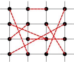
FIG. 1: An example of a lattice studied forL=4 (with periodic boundary conditions) showing both the regular square-lattice inter-actions (light lines, interaction strengthJ1) and a realization of the small world (random) interactions (heavy dashed lines). This corre-sponds to thez=5 lattice since every lattice site has fourJ1 interac-tions and one SW interaction of strengthJ2. (Color online.)
II. MODEL AND METHODS
The models studied here are Ising models withN=L2Ising
spins with si=±1 on a L×L square lattice with periodic
boundary conditions, and with a nearest-neighbor ferromag-netic interaction of strengthJ1. A fixed number of SW bonds
with interaction strengthJ2are added to the square-lattice (see
Fig. 1), by randomly picking pairs of atoms and connecting them with a bond. Note that once the pair of atoms is picked, these atoms are not allowed to be picked again until all atoms have been picked. In other words, every node will have a co-ordination numberz betweenzmax andzmax−1. The Ising
Hamiltonian is given by
H
=−J1∑
hi,ji
sisj−J2
∑
SWsisj−J3
∑
SW++We use either ‘normal’ SW bonds of strengthJ2, or else given
a SW bond of lengthℓbetween the randomly chosen atoms we string a chain ofℓ+1 atoms with interaction strengthJ3
between these chosen square-lattice atoms. We always set ei-therJ2orJ3equal to zero.
We will first study here in detail scaling of a model withz SW bonds per atom with J2=1 andJ1=J3=0. We will call
this model thez-model. It was first introduced by Scalettar [25] in 1991, before the introduction of SW networks. Never-theless, it corresponds to a particular SW lattice. In particular, it can be mapped onto a one-dimesional lattice withz−2 SW interactions. This model is studied to determine whether the scaling for it is that of [25] or of another form predicted by Br´ezin and Zinn-Justin [26] and utilized to study Ising sys-tems with long-range interactions [27–30].
We utilized standard Monte Carlo (MC) simulations [31], with the site for an attempted update chosen at random. We utilized a Glauber flip probability and the SPRNG [32] ran-dom number generator. In particular, if the next ranran-dom num-ber isrthe spin is flipped if
r≤ exp−
Enew/kBT
exp−Eold/kBT+exp−Enew/kBT (2) where Eold is the current energy and Enew is the energy if
the chosen spin is flipped. The temperature isT andkB is
Boltzmann’s constant (in our unitskB=1). For a system with N Ising spins, the units of time are Monte Carlo Steps per Spin (MCSS), which corresponds toNspin flip attempts. We measured a number of quantities, and report here on the or-der parameter|M|= 1
NK∑ K
j=1
¯ ¯∑Ni=1si
¯
¯j, as well as the integer moments of the magnetization
Mb® = 1
K∑ K
j=1
¡1 N∑
N i=1si¢
b j.
The summation index jruns over theK different configura-tions generated in the Monte Carlo simulation. From these moments the susceptibilityχT = N
kBT ¡
M2® − |M|2¢
and the Binder fourth-order cumulant U4=1− h
M4i
3hM2i2 were calcu-lated. Simulations were performed using up to 128 process-ing elements usprocess-ing trivial parallelization. Obtainprocess-ing points for thez-model for the largest system sizeN=2562took about 52 hours per data run. Averages for all runs used betweenK=106
and 108MCSS per point. The crossings for differentNvalues
forU4give the critical temperatureTc for each model [31].
These values are listed in Table I.
III. RESULTS AND SCALING:z-MODEL
In this section we present results for thez-model (J1=J3=0, J2=1) where every node has zrandom links. There are no
square-lattice interactions, and consequently this model maps onto a linear chain with every spin having one random (small-world) link ifz=3. This model also corresponds to the model introduced by Scalettar [25]. We studied the model for z values between 3 and 8, and simulated system sizes up to
J1 J2 J3 z Tc model 1 0 0 4 2.2691··· square lattice 0 1 0 2 0.0 z-model (linear chain) 0 1 0 3 1.821 z-model
0 1 0 4 2.885 z-model 0 1 0 5 3.914 z-model 0 1 0 6 4.933 z-model 0 1 0 7 5.942 z-model 0 1 0 8 6.950 z-model 1 1 0 5 3.791 SW-model 1 1 0 6 4.872 SW-model
1 4 0 5 5.391 SW-model 1 4 0 6 8.835 SW-model
TABLE I: Table 1. Values of the critical temperatureTcfor the var-ious models described in the text. All values are accurate within
±0.005. See the text for a full description of the models.
1 2 3 4 5 6 7 8
k
BT/J
0 0.1 0.2 0.3 0.4 0.5 0.6
U4
(a)
z=3 z=4 z=5 z=6 z=7 z=8
1 2 3 4 5 6 7 8
k BT/J 1
10 100
χ
T
N=64*64 N=128*128 N=256*256
z=3 z=4 z=5 z=6 z=7 z=8
(b)
FIG. 2: The Binder CumulantU4(a) andχT/N(b) is shown for the z-model (J1=J3=0, J2=1) forN=642, 1282, and 2562. In (a) the horizontal line isU4,∞(mf). The legend holds for both graphs. (Color online.)
N=2562=65536 (although the starting square-lattice struc-ture is unimportant for the z-model, we will still report the system size asN=L2).
Fig. 2 shows the values forU4 and χT for the z-model.
These figures also allow one to read off the value forTc. The
0 0.2 0.4 0.6 0.8 1 T/T
c
0 0.2 0.4 0.6 0.8 1
|M|
z=3 z=4 z=6 z=8 MF
FIG. 3: The magnetization per spin is shown for thez-model with N=2562. The solid line is the mean-field result of Eq. 3. (Color online.)
the solution of the equation M(T) =tanh
µ Tc
TM(T) 
. (3)
Note that aszincreases the curves for|M|approach that of the mean-field result.
The general form for scaling at a second order phase tran-sition as a function of the reduced temperature
t=|(T−Tc)/Tc| (4)
is given by [31]
χ=L−effγ/νf³L1/effνt´ (5) withγthe critical exponent forχandνthe critical exponent for the correlation length. Here the effective length that enters scaling,Leff, depends on the dimension of the system. For a
regulard-dimesional latticeLeff=N 1
d. However, this type of scaling does not hold for systems at or above the upper criti-cal dimension. These systems behave in a mean-field fashion, such as thez-model. Scalettar showed that the average sepa-ration of spins in thez-model is
ℓsep=a(z) +˜ b(z)˜ ln(N), (6)
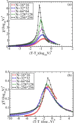
and suggested that scaling for the z-model should scale as in Eq. 5 withLeff∼ℓsep∼ln(N). His fit parameters (compare
Fig. 5 of ref. [25]) usedTc=1.87 and fits ofa=2 andb=1.887
in plots ofχ/[ln(N)]aversus(T−T
c)[ln(N)]b. Our data for the
same parameters are shown in Fig. 4(a). Note that the crossing ofU4with different system sizes actually gives a lower value
for Tc (Table I). Using the best fit parameters a and b for
data collapse scaling of our data forz=3 and the value ofTc
from theU4crossings gives the fit shown in Fig. 4(b). In
nei-ther case in Fig. 4 does the scaling look very good. Note that with the additional computer power available today, our sys-tem sizes and statistics are much greater than that of ref. [25].
-4 -3 -2 -1 0 1 2
(T-T
c)(log10V) b
0 1 2 3 4 5 6 7
χ
/(log
10
V)
a
N=16*16 N=32*32 N=64*64 N=128*128 N=256*256
(a)
-10 -8 -6 -4 -2 0 2 4
(T-T
c)(log10V) b
0 0.1 0.2 0.3 0.4 0.5
χ
T/(log
10
V)
a
N=16*16 N=32*32 N=64*64 N=128*128 N=256*256
(b)
FIG. 4: Scaling as in ref. [25] for thez=3 model, with the attempted scaling form of Eq. 5 withLeff=ln(N). In (a) the parameters of ref. [25] are used:Tc=1.870,a=2.0,b=1.8868. In (b) the best-fit parameters for the scaling form are used, withTc=1.821 given by the crossing of the Binder cumulant and the fit parametersa=4.1 andb=3.58. (Color online.)
In summary, thez-model does not scale as was proposed in 1991 in ref. [25]. To ensure that these results were accu-rate, each author developed independently a code for thez=3 model using different random number generators. Both codes gave comparable results, leading to a belief that our Monte Carlo data are indeed correct for this model.
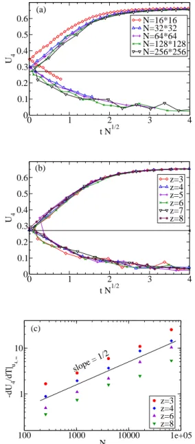
At and above the upper critical dimension, Br´ezin and Zinn-Justin in 1985 [26] predicted that the Ising model should scale such that for infinite system sizes the value of the Binder cumulant atTc should be equal toU4,(mf∞) ≈0.2705. As
ex-pected, this value is different from thed=2 Ising result of U4,(d∞=2)≈0.615 [31]. Furthermore, Br´ezin and Zinn-Justin pre-dicted that the mean-field systems should exhibit finite size scaling for small values of the reduced temperaturetwith
U4(t) = fU
³ tN12
´
(7) and taking derivatives with respect totgives
∂U4(t)
∂t =N 1
2 f′
U
³ tN12
´
0 1 2 3 4 t N1/2
0 0.1 0.2 0.3 0.4 0.5 0.6
U4
N=16*16 N=32*32 N=64*64 N=128*128 N=256*256 (a)
0 1 2 3 4
t N1/2 0
0.1 0.2 0.3 0.4 0.5 0.6
U4
z=3 z=4 z=5 z=6 z=7 z=8 (b)
100 1000 10000 1e+05
N 1
10
-dU
4
/dT
|u4,
∞
z=3 z=4 z=6 z=8 (c)
slope = 1/2
FIG. 5: The Binder 4th-order cumulantU4scaling for thez-model as given by Eq. 7 and 8. (a)z=3 for variousNvalues. (b)N=2562 for variouszvalues. (c) for variouszvalues dU4
dT evaluated at the predicted value ofU4,∞(mf). (Color online.)
They also predicted for smalltthe finite-size scaling form χT =N12 fχ
³ tN12
´
. (9)
Although not stated explicitly in their paper, their scaling form for the order parameter is
|M(t)|=N−14 fM ³
tN12 ´
(10) forT<Tc. The predicted scaling forU4and its derivative with
respect tot works extremely nicely for all values of zfrom z=3 to our largest studied valuez=8, as shown in Fig. 5. It
should be stressed that this scaling plot hasno adjustable pa-rameters, since the value forTcis obtained by the crossings
ofU4for various values ofN. Similarly, The exact mean-field
(mf) value forU4for the infinite lattice [26] is shown as the
horizontal lines. Fig. 6 shows the predicted scaling for var-ious values ofN andzfrom Eq. 9 for χT and from Eq. 10 for|M|, again with no adjustable parameters sinceTcis taken
from the crossings ofU4. Again the scaling is very good. The
asymptotic slopes for smallt and largeN with largetN12 for |M|in Fig. 6(a) is 12. This value can be seen since the scaling function gives
|M|=N−14 fM ³
tN12 ´
→N−14 ³
tN12 ´12
=t12 =tβ (11)
with the mean field value for this exponent isβ=12. Similarly, since the mean field value of the susceptibility exponent is γ=1 the asymptotic slope in Fig. 6(b) should be −1. Most of the spread in the scaling in Fig. 6 is a vertical shift of the curves for various values of z. This may be due to one or more of several reasons. One possibility would be slight errors in the values ofTc, perhaps caused by different convergence
rates with different zto the infinite lattice values. Another possibility would be that the prefactor for|M|andχT atTcfor
finiteNis slightly different. Our data at this point is not of a sufficient quality to decide among these possible alternatives. Nevertheless, the scaling predicted by Br´ezin and Zinn-Justin [26] is seen to hold.
IV. RESULTS AND SCALING: SW-MODEL
This section presents results for scaling for the normal small-world model (SW-model). This hasJ1=1, J3=0, and
a non-zero positive value forJ2. Every spin has four
nearest-neighbor ferromagnetic interactionsJ1due to the underlying
square-lattice structure. We will study the case where every spin has one SW bond and hencez=5, and the case where every spin has two SW bonds and hencez=6. From the cross-ings ofU4for various values ofNwe obtain the values of the
critical temperature listed in Table I. Fig. 7 shows that the anticipated form for the scaling ofU4from Eq. 7 and of the
derivative ofU4with respect tot from Eq. 8 provides
excel-lent data collapse scaling for various values ofzandNand for both the studied values ofJ2: J2=1 andJ2=4. The thickness
of the region of data collapse seems to be more from the sta-tistical properties of the data, or from small errors inTc, than
from a lack of scaling or of corrections to scaling. Fig. 8(a) shows the scaling predicted from Eq. 10 for the order parame-ter|M|, and Fig. 8(b) shows the data collapse scaling forχT from Eq. 9. In both cases the data collapse is very good for both values ofJ2, for bothz=5 andz=6, and for both system
0.1 1 10 tN1/2
0.1 1 10
|M| N
1/4
N=128*128, z=3 N=256*256, z=3 N=128*128, z=4 N=256*256, z=4
(a)
slope = 1/2
slope = -1/2
0.1 1 10
tN1/2 0.01
0.1 1
χ
T/N
1/2
N=128*128, z=6 N=256*256, z=6 N=128*128, z=8 N=256*256, z=8 (b)
slope = -1
FIG. 6: Scaling versustN12 for thez-model for various values ofz andN=1282and 2562. (a) Magnetization:MN14. (b) Susceptibility: χT N−12. Both legends list symbols for data in both graphs. (Color online.)
system sizes demonstrates corrections to scaling, and conse-quently only our largest two system sizes are shown in these scaling figures. Again, it must be emphasized that since the value forTc is taken from the crossings ofU4 the curves in
Fig. 7 and Fig. 8 haveno adjustable parameters.
The underlying scaling behavior of the SW model with z=5 andz=6 is consistent with other studies of Ising mod-els with SW interactions (usually starting fromd=1) models [11–13, 15, 16, 18, 20, 22–24]. Consequently, these mod-els have a critical behavior with mean-field critical exponents γ=1,β=1
2,α=0, andν= 1
2(but as in the comment to Ref. [13]
with ¯ν=2−α=2).
There is also a prediction [17] that in the N→∞limit the order parameter should scale forT<Tcas
|M|=A˜√Tc−T (12)
with the mean field amplitude ˜A∝p
βd=2−βmf
γd=2 diverging as the
strength of the SW couplings p approaches zero. In [17] it is argued that this behavior will also be seen as the number of SW bonds becomes small, i.e. when z=4+p→4 for our square-lattice model. We have simulated our square-lattice model forz=5 with weakJ2=0.01,0.05,0.1,0.5 for system
sizes up toN=3842. However, we were not able to obtain the
0 1 2 3 4
t N1/2 0
0.1 0.2 0.3 0.4 0.5 0.6
U4
N=128*128, J2=1, z=5 N=256*256, J2=1, z=5 N=128*128, J2=1, z=6 N=256*256, J2=1, z=6 N=128*128, J2=4, z=5
N=256*256, J2=4, z=5 N=128*128, J2=4, z=6
N=256*256, J2=4, z=6 (a)
100 1000 10000 1e+05
N 1
10
-dU
4
/dT
|u4, ∞
J2=1, z=5 J
2=1, z=6
J2=4, z=5 J2=4, z=6 (b)
slope = 1/2
FIG. 7: The Binder 4th-order cumulantU4scaling for the SW-model (J1=1, J3=0) forz=5 andz=6 for variousN values and for both J2=1 andJ2=4. (a)U4= fU(tN
1
2)from Eq. 7 withN=1282 and N=2562. The horizontal line the theoretical prediction forU4,∞(mf)and (b)dU4
dT evaluated at the predicted value ofU
(mf)
4,∞ from Eq. 8. (Color online.)
predicted scaling. To see this scaling requires that the width of the mean field region, which is [17] within
|Tc−T|∝p 1
γd=2 ∝|T
c−T¯c,d=2|, (13)
be sufficiently probed by the system size that finite size effects are negligible. It would be interesting to have a prediction for how finiteNwould manifest itself in this scaling. Computer simulations for SW systems with varying strengthsJ2 have
also recently been reported [20].
We have also investigated the case where the number of SW connections goes to zero asN increases. This study is motivated by physical small-world networks [22–24] where the number of short-cut bonds (which are SW bonds) can-not grow as fast as N. In [22, 23] it was shown that the properties of such systems for smallNcan nevertheless show some of the mean field properties of a full small-world sys-tem. Fig. 9 showsU4 for both the pure square-lattice Ising
model (z=4) and the SW model withz=4+√2
N. For the SW
model withz=4+√2
N asN→∞the pure square lattice results
0.1 1 10 tN1/2
0.1 1 10
|M| N
1/4
N=128*128, J2=1, z=5 N=256*256, J2=1, z=5 N=128*128, J2=1, z=6 N=256*256, J2=1, z=6
(a)
slope = 1/2
slope = -1/2
0.1 1 10
tN1/2 0.01
0.1 1
χ
T/N
1/2
N=128*128, J2=4, z=5 N=256*256, J2=4, z=5 N=128*128, J2=4, z=6 N=256*256, J2=4, z=6
(b)
slope = -1
FIG. 8: The scaling versustN12 for the for the SW-model forz=5 andz=6, forJ2=1 andJ2=4, forNvalues of 1282and 2562. . (a) Magnetization:MN14 from Eq. 10. (b) Susceptibility:χT N−
1 2. from Eq. 9. Both legends list symbols for data in both graphs. (Color online.)
256 SW bonds of strength J2=4 forN=2562=65536 spins
the temperature value whereU4changes from about23to zero
is shifted by about 5%. This indicates that even a vanishing fraction of SW bonds can have effects on the behavior of the system. This is demonstrated in the scaling of|M|in [23].
V. RESULTS AND SCALING: PHYSICAL SW-MODEL
There are two ways to obtain physical SW networks [22– 24] to study the effect of SW bonds that can be built from physical building blocks. These physical SW networks must satisfy certain constraints so that they can be built from phys-ical building blocks. These building blocks may be atoms, beads necklaces [23], or ball-and-stick models of atoms. One way to obtain physical SW networks is to have a vanishing number of SW bonds (short-cuts) asN increases. This was discussed in the previous section. The second way to obtain a physical SW network is to build the SW bonds from the un-derlying building blocks. This was done in [22] starting from ad=1 chain. Each SW bond is then composed of a string of spins with ferromagnetic coupling constantJ3, with the
num-ber of spins along the chain equal to the Euclidean distance between the randomly chosen sites. In [23] it was shown that
2.2 2.3 2.4 2.5 2.6 2.7
k
BT/J
0 0.1 0.2 0.3 0.4 0.5 0.6
U4
N=64*64, Pure Sq N=128*128, Pure Sq N=256*256, Pure Sq
(a)
0 2 4 6 8 10 12 14 16
t L1/ν (ν=1.0) 0
0.1 0.2 0.3 0.4 0.5 0.6
U4
N=64*64, SW J2=4 N=128*128, SW J2=4 N=256*256, SW J2=4
(b)
FIG. 9: The Binder 4th-order cumulantU4for the SW-model (J1=1, J3=0). This is both with no small-world interactions (pure square-lattice Ising model) (J2=0), and withLsmall-world interactions with J2=4 (z=4+2NL). The horizontal line isU
(d=2)
4,∞ for thed=2 Ising model (dashed). (a) showsU4versusT and (b) shows the predicted scaling with thed=2 value ofν=1. Both legends list symbols for data in both graphs. (Color online.)
the total number of spins in the d=1 case starting with N0
spins goes asNtot∝N02. For a d=2 model on aL2lattice the
total number of spins needed for every initial spin to also have a SW bond is expected to beNtot∝L3. This severely limits the
system size that can be simulated. We studied only system sizes up toL2=962=9216 in this section, which corresponds toNtot=185635 total Ising spins.
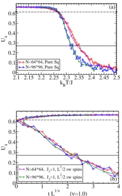
Here we present results for the physical SW model with J2=0 andJ1=J3=1. Fig. 10 showsU4and the scaling ofU4.
The SW bonds are built from linear chains of Ising spins. The linear Ising model does not have a finite temperature critical point. Consequently, one expects from renormalization group arguments that the critical exponents should be those of the d=2 Ising model. Furthermore, one expects that the critical temperature should be the same as for the square lattice Ising model,Tc= 2J1
ln(1+√2)≈2.269J1. Fig. 10(a) shows that indeed
2.1 2.15 2.2 2.25 2.3 2.35 2.4 2.45 2.5 kBT/J
0 0.1 0.2 0.3 0.4 0.5 0.6
U4
N=64*64, Pure Sq N=96*96, Pure Sq
(a)
0 1 2 3 4
t L1/ν (ν=1.0) 0
0.1 0.2 0.3 0.4 0.5 0.6
U4
N=64*64, J3=1, L2/2 sw spins
N=96*96, J3=1, L 2
/2 sw spins (b)
FIG. 10: The Binder 4th-order cumulantU4 for the physical-SW-model (J1=1, J2=0, J3=1) with N2 physical-small-world interac-tions. (a) Values of U4 versus T. The horizontal lines are the predicted values forU4,∞(mf) for the mean-field model (solid) and of U4,∞(d=2)for thed=2 Ising model (dashed). (b) The predicted scaling ofU4with the square-lattice Ising exponentν=1 and the square lat-tice Ising value (z=4) ofTc. Both legends list symbols for data in both graphs. (Color online.)
VI. DISCUSSION AND CONCLUSIONS
The Ising ferromagnet on models starting from the square lattice Ising model has been studied. The first conclusion, which has also been reached by other researchers, is that the Ising model with ‘normal’ small world (SW) bonds exhibits mean field scaling [Fig. 7 and Fig. 8].
We have investigated in detail thez-model of ref. [25], and found that the scaling form for χT is given by Eq. 9 from
[26] [Fig. 6(b)] rather than Eq. 5 withLeff=ln(N)postulated
in [25] [Fig. 4]. The scaling of ref. [26] [Eq. 7 through Eq. 10] also workswithout any adjustable parametersfor thez-model for other quantities such as the Binder cumulantU4[Fig. 5]
and the order parameter|M|[Fig. 6(a)]. Scaling as predicted forN→∞predicted in ref. [17] for a low density or for weak SW bonds could not be seen in our data. This most likely is because the finite size effects for theN values we studied obscured the predicted scaling.
We have also investigated the Ising model on physical SW networks starting from an underlying N=L2 square lattice.
The physical SW networks either have a number of SW bonds that vanish asN→∞(herez=4+√2
N), or are constructed from
a linear chain of spins with the number of spins along the chain equal to the Euclidean distance between the randomly chosen spins on the square lattice. The study here can be compared to physical SW studies in [22–24], as well as the study with power-law SW bond strengths [18]. The summary is twofold. First, physical SW bonds do not change the criti-cal properties of the model asN→∞. Second, the physical SW bonds have some effect on the scaling properties. They lead to much slower approaches to theN→∞results. They also show a regime near the effectiveTc,N, given by the
tempera-ture where for finiteN the value ofU4 quickly changes
be-tween23and zero, which shows some properties of mean field behavior. This is illustrated in [Fig. 9 and Fig. 10] and seen in [22, 23]. These type of SW connections have been used as models of liquid and amorphous selenium [33]. Conse-quently, the current study provides further evidence that phys-ical (quasi-) SW nanomaterials may exhibit mean field erties in both their critical behavior and in their transport prop-erties.
VII. ACKNOWLEDGEMENTS
We acknowledge useful discussions with a number of people, particularly Gyorgy Korniss, Per Arne Rikvold, and Zoltan Toroczkai. Supported in part by NSF grants 0120310, 0113049, 0426488, and DMR-0444051. Computer time from the Mississippi State Univer-sity High Performance Computing Collaboratory (HPC2) was
critical to this study.
[1]Low Dimensional Conductors and Superconductors, NATO ASI Series B, Phys. Vol. 155, editor D. Jerome and L.G. Caron (Plenum, New York, 1987).
[2] M.A. Novotny, Phys. Rev. B46, 2939 (1992). [3] M.A. Novotny, Phys. Rev. Lett.70, 109 (1993).
[4] G. Chartrand,Introductory Graph Theory, (Dover, New York, 1985).
[5] R. Albert and A.-L. Barab´asi, Rev. Mod. Phys.74, 47 (2002). [6] G. Korniss, M.A. Novotny, H. Guclu, Z. Toroczkai, and P.A.
Rikvold, Science299, 677 (2003).
[7] G. Korniss, M.A. Novotny, and P.A. Rikvold, J. Comp. Phys.
153, 488 (1999).
[8] G. Korniss, Z. Toroczkai, M.A. Novotny, and P.A. Rikvold, Phys. Rev. Lett.84, 1351 (2000).
[9] A. Kolakowska, M.A. Novotny, and G. Korniss, Phys. Rev. E
67, 046703 (2003).
[10] G. Korniss, M.A. Novotny, P.A. Rikvold, H. Guclu, and Z. Toroczkai, Materials Research Society Symposium Proceed-ings Series Vol. 700, p. 297 (2002).
[12] A. Barrat and M. Weigt, Eur. Phys. J. B13, 547 (2000). [13] A. Pekalski, Phys. Rev. E 64, 057104 (2001); comment H.
Hong, B.J. Kim, and M.Y. Choi, Phys. Rev. E 66, 018101 (2002).
[14] B.J. Kim, H. Hong, P. Holme, G.S. Jeon, P. Minnhagen, and M.Y. Choi, Phys. Rev. E64, 056135 (2001).
[15] H. Hong, B.J. Kim, and M.Y. Choi, Phys. Rev. E66, 018101 (2002).
[16] C.P. Herrero, Phys. Rev. E65, 066110 (2002). [17] M.B. Hastings, Phys. Rev. Lett.91, 098701 (2003).
[18] D. Jeong, H. Hong, B.J. Kim, and M.Y. Choi, Phys. Rev. E68, 027101 (2003).
[19] B. Kozma, M.B. Hastings, and G. Korniss, Phys. Rev. Lett.92, 108701 (2004).
[20] D. Jeong, M.Y. Choi, and H. Park, Phys. Rev. E71, 036103 (2005).
[21] B. Kozma, M.B. Hastings, and G. Korniss, Phys. Rev. Lett.95, 018701 (2005).
[22] M.A. Novotny and S.M. Wheeler, Braz. J. Phys.34, 395 (2004). [23] A.M. Novotny, X. Zhang, T. Dubreus, M.L. Cook, S.G. Gill,
I.T. Norwood, and G. Korniss, J. Appl. Phys. 97, 10B309 (2005).
[24] M.A. Novotny, inComputer Simulation Studies in Condensed Matter Physics XVII, editors D.P. Landau, S.P. Lewis, and H.-B. Sch¨uttler, (Springer, Berlin), in press.
[25] R.T. Scalettar, PhysicaA170, 282 (1991).
[26] E. Br´ezin and J. Zinn-Justin, Nucl. Phys. B257, 867 (1985). [27] E. Luijten and H.W.J. Bl¨ote, Phys. Rev. Lett.76, 1557 (1996). [28] M. Laradji, D.P. Landau, and B. D¨unweg, Phys. Rev. B51, 4894
(1995).
[29] E. Luijten and K. Binder, Phys. Rev. E58, R4060 (1998). [30] E. Luijten, Phys. Rev. E60, 7558 (1999).
[31] D.P. Landau and K. Binder,A Guide to Monte Carlo Simula-tions in Statistical Physics(Cambridge University Press, Cam-bridge, UK, 2000).
[32] See http://sprng.cs.fsu.edu