ABSTRACT: The sensitivity of the planetary boundary layer (PBL) parameterizations is investigated using the hybrid Fifth Generation Penn State University/National Center for Atmospheric Research (NCAR) Mesoscale Model (MM5) and its results were compared with observations from two ield campaigns held during the dry and wet seasons at the Centro de Lançamento de Alcântara (CLA). The comparisons were made using the integrated zonal and meridional components of observed and forecasted winds. Initially, three boundary layer parameterizations, in addition to the current parameterization, were selected for evaluation: Blackadar (BLK), Medium Range Forecast (MRF), Janjic (ETA) and Burk-Thompson (BT). The MRF and BLK schemes produced better results than the ETA and BT schemes. Nevertheless, MRF and BLK underestimate the zonal and meridional wind components by around 16% in the rainy season and overestimate them by on average 18% in the dry season.
KEYWORDS: Centro de Lançamento de Alcântara, MM5, Boundary layer parameterizations.
The Sensitivity of Wind Forecasts with a
Mesoscale Meteorological Model at the
Centro de Lançamento de Alcântara
Elizabeth Diane de Jesus Reuter1,2, Gilberto Fisch3, Cleber SouzaCorrea4
INTRODUCTION
Nowadays, in the ield of Aerospace Meteorology, atmospheric modeling and numerical simulations are necessarily present in the operational planning and logistics of space vehicle launches, with the goals of guaranteeing higher security in the activities on the surface and in light and thus contributing to the success of the launches. he Aerospace Meteorology is the application of atmospheric science towards the design, development, and operation of aerospace vehicles. At the Centro de Lançamento de Alcântara (CLA), it supports the observation missions and analysis of climate elements at the surface and altitude, as well as produces the weather forecast.
An aerospace vehicle’s response to atmospheric disturbances, especially wind, must be carefully evaluated to ensure that the design will meet its operational requirements (Johnson, 2008). A large number of diferent Numerical Weather Prediction models have been utilized in the operational sectors of Meteorology as a work tool. However, the limitations of each of them mean that, for each particular problem, it is necessary to develop or modify a code according to the speciic desired requirements. In the case of rocket launches at the CLA, the search for a model capable of predicting the shear and wind proile with antecedence of hours in a large area of ocean-continent transition is very important given the operational necessity of understanding the winds for the determination of the vehicle trajectory and for studies of dispersion of the gases liberated by rocket combustion processes at the surface level at the launch pad.
1.Instituto Nacional de Pesquisas Espaciais – Centro de Previsão de Tempo e Estudos Climáticos – São José dos Campos/SP – Brazil. 2.Secretaria da Aviação Civil – Empresa Brasileira de Infraestrutura Aeroportuária – Guarulhos/SP – Brazil. 3.Departamento de Ciência e Tecnologia Aeroespacial – Instituto de Aeronáutica e Espaço – Divisão de Ciências Atmosféricas – São José dos Campos/SP – Brazil. 4.Departamento de Controle do Espaço Aéreo – Instituto de Controle de Tráfego Aéreo – Rio de Janeiro/RJ – Brazil. Author for correspondence: Gilberto Fisch | Instituto de Aeronáutica e Espaço – Divisão de Ciências Atmosféricas | Praça Marechal Eduardo Gomes, 50 – Vila das Acácias | CEP: 12.228-901 – São José dos Campos/SP – Brazil | Email: [email protected]
Although each physical parameterization package in a mesoscale model plays an important role in atmospheric simulations, the parameterizations of the planetary boundary layer (PBL) are formulations more simple than the complex physical processes that occur in the nearest layers of the Earth’s surface. For better understanding, some deinitions are important such as: mesoscale is the scale of meteorological phenomena that ranges in size from a few km to about 100 km. It includes local winds, thunderstorms, and tornadoes. PBL is the bottom layer of the troposphere that is in contact with the surface of the Earth. It is oten turbulent and is capped by a statically stable layer or temperature inversion of air. Surface boundary layer (SBL) is the layer of air of order tens of meters thick adjacent to the ground where mechanical (shear) generation of turbulence exceeds buoyant generation or consumption.
he PBL parameterizations are mathematical formulations simpler than the complex physicals processes that occur in the layers closest to the Earth’s surface. he principal process is turbulence, which is responsible for the vertical distribution of the properties related to heat surface luxes, moisture and momentum within the PBL.
The realistic importance, in other words, the faithful representation of the existing processes in the PBL and SBL in meteorological models, is out of question, principally in mesoscale models. It should be taken into consideration because the majority of these parameterizations were developed based on measurements and studies conducted in Northern Hemisphere mid-latitude locations, principally in the United States and Europe. hus, it is necessary to study the inluence of these schemes on the simulation of meteorological variables in other regions, particularly in the equatorial region. here are relatively few validation studies of numerical weather models for the equatorial region: for instance, Oyama (2004), in a preliminary study, evaluated the sensitivity of the MM5 model to the deep convective parameterizations on reduced grids; Oyama and Giarolla (2006) simulated squall lines on the northern coast of Brazil also using the MM5 model. hese simulations were performed in order to verify the ability of the model to represent the life cycle of squall lines (LI) initiated in the northern coast of Brazil. Squall line is a line of active thunderstorms, either continuous or with breaks, including contiguous precipitation areas resulting from the existence of the thunderstorms. he MM5 satisfactorily represented the life cycle of LI and, as a consequence, the weather; Pereira Neto and Oyama (2011) proposed adjustments in the Kain-Fritsch
(KF2) deep convective parameterization scheme with the goal of improving precipitation prediction at the CLA. With the adjustments, a marked improvement in the representation of the total precipitation and of the monthly fraction of rainy days was found.
he spatial pattern of errors in the ield, however, has not undergone many changes over the continent and, in general, rainfall is best represented over land than over ocean. Also using the MM5 regional model, Carvalho (2011) tested the sensitivity of simulated precipitation to diferent schemes of explicit convection, the activation of shallow convection (Grell, 1993) and adjustments in the scheme of deep convection KF2 scheme. Adjustments in KF2 comprehended changes in minimum depth of cloud required to activate the convection in the parameters “trigger” function and convective scales of advective and convective weather. The modeling study showed that the use of explicit convection “warm rain” and shallow convection schemes of Grell along with the “in line” in KF2 substantially reduced the overestimation of precipitation found in the simulations for the operating region of the Intertropical Convergence Zone — the axis, or a portion thereof, of the broad trade-wind current of the Tropics (ITCZ). All of these studies contributed to a better understanding of how to utilize atmospheric mesoscale modeling, in particular, the MM5 model, at the CLA region in order to support the launchings. However, they did not address the ability of the mesoscale model to forecast winds. he rainfall and the winds, both at surface and upper air, are the two key-parameters for the launchings of Brazilian rockets at CLA.
So, in order to use a numerical model to forecast the winds at the CLA, this study addressed the question of its evaluation using four diferent PBL parameterizations, to be described in section Description of the Modiied MM5 Model, against data sets collected by radiosonde winds from the surface up to 5,000 m during wet and dry periods.
DATA
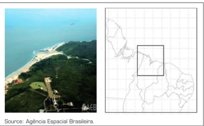
Figure 1. Aerial view of the CLA and grids with horizontal resolutions of 18 km (larger domain) and 6 km
(smaller domain).
Source: Agência Espacial Brasileira.
he data were obtained from two ield campaigns: Operation Murici 2008, during the dry season of 2008, and GPM 2010, wet season of 2010, and consist of systematic radiosounding launched at 00, 06, 12 and 18 UTC, during the periods from September 16–26, 2008, characterizing the dry season, to from March 19–25, 2010, characterizing the wet period. Meteorological parameters such as pressure, temperature and humidity were measured by the radiosonde in situ sensors while the direction and wind speed were determined by the GPS satellite navigation. he radiosonde soundings were performed using equipment model Vaisala OY (DigiCORA) using the sondes RS80-15G and RS92-SVP in experiments in 2008 and 2010, respectively.
DESCRIPTION OF THE MODIFIED MM5 MODEL
In this study, the hybrid Fifth Generation Penn State University/National Center for Atmospheric Research (NCAR) Mesoscale Model (MM5) (Grell et al., 1994; Dudhia et al.,
2003) was utilized. he model is for numerical simulation of the atmosphere and was developed in the late 1970s by Penn State University, in conjunction with the National Center for Atmospheric Research (PSU/NCAR). In Brazil, the Laboratório de Prognósticos em Mesoescala (LPM) of the Departamento de Meteorologia of the Universidade Federal do Rio de Janeiro (UFRJ) provides predictions for the state of Rio de Janeiro with 20 km resolution. he Instituto de Controle do Tráico Aéreo (ICEA), on the other hand, in partnership with the Centro Nacional de Meteorologia Aeronáutica (CNMA), both subordinated to the Departamento de Controle do Espaço Aéreo (DECEA) and the IAE of Departamento de Ciência e Tecnologia Aeroespacial (DCTA), uses the MM5 model with objectives of research and operational numerical modeling for
aeronautical and space vehicle. he numerical simulation tests were conducted in the ICEA/DECEA research facility, which is located within the DCTA.
As the model was developed in order to simulate or predict atmospheric circulation, it is supported by pre- and post-processing programs. he MM5 model is a limited area model, which needs lateral boundary conditions to represent the real state of the atmosphere neighboring the simulation domain through the time of integration of the dynamic equations. hese boundary conditions are obtained through a global scale atmospheric model, for example, the Global Forecast System (GFS), obtained from the address: http://www.ncdc.noaa.gov/data-access/model-data/ model-datasets/global-forcast-system-gfs.
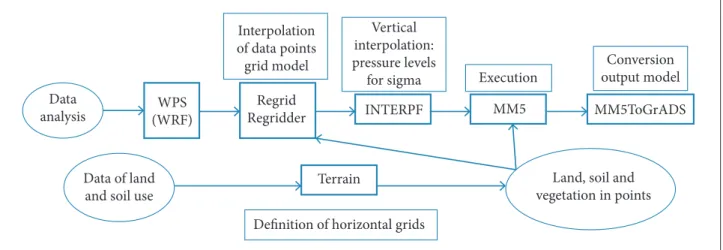
The modeling system consists of a set of components necessary to run the model: the Pre-processing System (WPS), the pre-processing package used in the Weather Research and Forecasting (WRF) Model, which horizontally interpolates the meteorological variables of geopotential height, wind, temperature and mixing ratio in each isobaric level, temperature and pressure on the surface and temperature and humidity of the soil layers; in this way, the version used MM5 can be considered hybrid format GRIB2. In this version of MM5, the REGRID package horizontally interpolates the analyzes and forecasts, the INTERPF vertically interpolates the pressure to sigma coordinates and also generates the initial and boundary conditions; in MM5, there are the parameter definitions, implementation of the model and periods of integration and assimilation of data and MM5toGrADS is done post-processing, which generates converted output to GrADS format. In this way, the version of MM5 used can be considered hybrid format GRIB2. Figure 2 depicted the flow chart of MM5.
This study considers the following parameterizations: Blackadar (BLK), described by Zhang and Anthes (1982), Burk-hompson (BT; Burk and Burk-hompson, 1989), ETA (Mellor and Yamada (1974); Janjic (1994) and Hong-Pan (Medium Range Forecast - MRF); Hong and Pan, 1996) PBL schemes available in the MM5 model, in agreement with Table 1.
Figure 2. Flowchart of operation of the hybrid mesoscale model MM5.
Name Abbreviation Original scheme
Closure order
Theory for vertical turbulent diffusion
Vertical diffusion
Surface layer similarity
Blackadar BLK Blackadar First order K-theory non-local Monin-Obhukov
Burk-hompson B-T Mellor-Yamada Second
order TKE local Louis
Mellor-Yamada ETA Mellor-Yamada Order 1.5 TKE local Monin-Obhukov
Hong-Pan MRF Troen-Mahrt First order K-theory non-local Monin-Obhukov
Table 1. PBL parametrization schemes tested in MM5.
Source: Adapted from Camillo (2011).
convection, the heat exchange, humidity and momentum occur through mixing between elements originating at the surface and the environmental air PBL. he stable regime, also known as nighttime, and the unstable regime are treated diferently: in the nighttime, the atmosphere is stable or lightly unstable and turbulence is the result of mechanical processes, while during the daytime, or free convection regime, the atmosphere is unstable and the turbulence is the result of free convection of thermals of rising hot air, associated with the mechanical processes wind shear. In the nocturnal regime, a irst order closure based on K theory approximationis used to determine the turbulent luxes. K theory approximation, also called mixing-length theory, is a method of describing the movement of trace species on the turbulent or subgrid scale; the theory relates the luxes of the trace species to the gradient of the mean quantities via eddy difusivity denoted K. Considering the nocturnal regime as a local scheme, the mixture is assumed to occur only between adjacent layers in the model. he free convection regime employs a non-local approximation in which buoyancy plumes of hot air are assumed for the mixing of heat, humidity and momentum for each level in the mixing layer.
he B-T scheme available in MM5 is based on its initial implementation in NORAPS (Burk and hompson, 1989). The PBL turbulence parameterization scheme with local second order closure is based on level 3 of Mellor and Yamada (1974). In the MM5 model, this scheme is used to predict the vertical mixing of horizontal wind, potential temperature, water vapor mixing ratio, cloud water and rain water through prognostic equations for the turbulent kinetic energy (TKE), temperature, humidity and a covariance of temperature and humidity. All other lows are obtained diagnostically. heir inclusion in the prognostic equations for larger statistical moments permits the simulation of better mixed PBLs, but with a large computational increase. It is a local closure PBL scheme of order 1 and ½ with a prognostic equation for turbulent kinetic energy.
The parameterization based on modeling developed by Janjic (1994), which will be called from here only as ETA, uses equations defined by Mellor and Yamada (1974), who consider the closure of second-order turbulence for the TKE and calculate the turbulent fluxes from it. According to Janjic (1994), this model assumes two distinct layers in PBL: a thin viscous layer above the surface, where the vertical transport
Data analysis
Data of land and soil use
Land, soil and vegetation in points Vertical
interpolation: pressure levels for sigma Interpolation
of data points
grid model Conversion
output model Execution
Terrain
Deinition of horizontal grids WPS
(WRF) MM5 MM5ToGrADS
Regrid
is determined by molecular diffusion, and a turbulent layer, where the vertical transport is dominated by turbulent flows. The thickness of the viscous layer is different relative to the temperature, specific humidity and wind speed and depends on the friction of its molecular diffusivity of each variable (Reynolds number). Additionally, viscous layers for temperature and humidity respectively depend on the Prandtl and the Schmidt numbers. These layers are much thinner than the surface layer. The turbulent flows of the different variables in the surface layer above the viscous layer are equal to those of the viscous layer and function of the gradient of these variables and coefficients of heat exchange and momentum defined by Mellor and Yamada. In MM5, the scheme is used to predict the vertical mixing of horizontal wind, potential temperature and mixing ratio.
An eicient scheme named MRF based on the Troen-Mahrt representation of the contragradient term and non-local K approximation (Hong and Pan, 1996) is a non-local scheme of irst order based on results from large eddy simulations by Wyngaard and Brost (1984). In this scheme, there is a low parametrization contrary to the gradient, which depends on the convective velocity and the low to the surface. It has been used in general circulation and numerical weather prediction models due to its computational eiciency. In the MM5 model, the scheme is used to predict the vertical mixing of horizontal wind, potential temperature, water vapor mixing ratio, cloud water and cloud ice.
DESCRIPTION OF THE EXPERIMENTS
he initial and boundary conditions for the simulations were based on data from the Global Forecast System (GFS) global model. he model integrations were initialized using the 12 UTC analyses and extended for 72 hours. he irst 12 hours of the simulation were not evaluated and the results were discarded as spin-up. he zonal (u) and meridional (v) wind components simulated were obtained for the grid point location closest to the CLA, whose coordinates are 2.23039° S and 44.4617° W. hese variables are compared with the observations derived from radiosoundings. he wind analysis is done in the lower atmosphere; in this case, from the surface to 700 hPa, this is equivalent to a height up to 5,000 meters, because these are the altitudes where there are the largest rocket trajectory corrections.
Also, other additional input data are:
• Frequency of boundary conditions is that established by analysis and forecast iles obtained from theNational
Centers for Environmental Prediction (NCEP) site. For MM5, iles were obtained every 6 hours.
• Atmospheric information to the initial conditions: GFS analysis and forecasts. he program WPS, the WRF system, is used to read iles in GFS format GRIB2 because the program responsible for this task only reads the MM5 format GRIB1.
• Sea surface temperature (SST) to the boundary condi-tions: the issue of SST is one aspect that still remains to be implemented in hybrid MM5. herefore, the surface temperature was used in place of SST, given that this comes from the GFS ile and is processed by the WPS.
• Moisture and soil temperature to the boundary conditions: these conditions were obtained from the GFS ile.
he tested coniguration of the MM5 can be summarized as: two domains nested; horizontal grid spacing of 18.6 km; number of the points of the domain size — 130 x 130, 121 x 121; 26 vertical levels and initialization at 12:00 UTC using GFS data. For the comparison of results, the parameterization MRF PBL was considered as reference or control and three other PBL parameterization options like BLK, ETA and BT were varied.
he physical parameterizations of the model are as follows: cloud radiation scheme for radiation; processes for multilayer surface; Grell for convection implied (Grell, 1993), which considers only a cloud-sized two-dimensional parameterization of vertical downward and upward movements and considers that there is only air mixture saturated with air at the top and the cloud base; simple ice (Dudhia, 1989) for cloud microphysics, which states that processes associated with the ice phase are more important in a layer between 0° and -20°C, where the vertical movements are forced to rise by releasing latent heat that results from deposition of water vapor in the snow.
METRIC FOR THE EVALUATION OF THE MM5 MODEL
In order to analyze the correlation of the simulation data in relation to the observations, the Willmott coefficient d
r (Willmott et al., 2011) was utilized according to Eqs. 1 and 2. It can be calculated as:
If
(1a)
Interval Performance
1.0 to 0.75 Excellent
0.75 to 0.5 Good
0.5 to 0.25 Reasonable
0.25 to -0.25 Fair
-0.25 to 0.5 Unsatisfactory
-0.5 to -0.75 Poor
-0.75 to 1.0 Very poor
Table 2. Evaluation criteria adopted by Willmott.
where: P
i: estimated value of a variable of order i; Oi: observed value of a variable of order i; Ō: mean of the estimated values of a variable; n: number of events.
he value of c was assumed as 2, according to Willmott et al. (2011).
he interpretation of d
r is relatively simple: it indicates the
sum of the magnitudes of the diferences between the deviations of the model and observed values about the observed mean in relation to the sum of the magnitudes of the perfect model (P
i = Oi, for all i) and the observed deviations about the observed mean. Since the Willmott index can vary in the interval of -1.0 to 1.0, here the evaluation criteria presented in Table 2 were considered.
he evaluation of the simulation is divided into two parts. First, a purely graphical comparison was made between the results obtained from the simulations, so considering each type of CLP parametrization with the observed value and also comparing with the NCEP reanalysis (Figs. 3 to 6). In the second part, the statistical metric Willmott index of agreement was used in the analysis, considering every 12 hours in advance prediction regarding the observation, namely, 60, 48, 36, 24 and 12 hours before the event.
GRAPHIC ANALYSIS
Year 2008
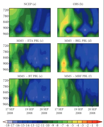
Considering for September 17, 2008 a booting from 12:00 UTC (Fig. 3), the ETA simulations (Fig. 3c), BLK (Fig. 3d), BT (Fig. 3e) and MRF (Fig. 3f) tend to overestimate, especially ETA and BT parameterizations, the zonal wind above 925 hPa. The startup from 12:00 UTC did not result in better forecasting for the meridional component (Fig. 4). It was noticed a change in the sign of the meridional component from 1,000 to 700 hPa, where, in the lower levels, the value
RESULTS
In this section, we will try to identify the main diferences between the parameterizations of PBL with respect to the ability of the model to predict 60 hours of wind in terms of zonal (u) and meridional (v) components. he irst 12 hours are not assessed and they are discarded as spin-up time efect. he two periods were analyzed as dry period of 2008 since 17 September at 12:00 UTC until 21 September at 12:00 UTC and as rainy period of 2010 since 19 March at 12:00 UTC until 25 March at 12:00 UTC.
Figure 3. Example of comparisons of the zonal wind component (m/s) between 1,000 and 700 hPa. (a) Reanalyses - NCEP; (b) Radiosoundings at CLA; MM5 simulations utilizing the ETA (c), BLK (d), BT (e) and MRF (f) parametrizations.
960 720 780 840 900
960 720 780 840 900
960
17 SEP 2008 17 SEP
2008
19 SEP 2008
20 SEP 2008
19 SEP 2008
20 SEP 2008
720 780 840 900
NCEP (a) OBS (b)
MM5 – ETA PBL (c) MM5 – BKL PBL (d)
MM5 – BT PBL (e) MM5 – MRF PBL (f)
-18-17 -16-15-14-13 -12-11-10 -9 -8 -7 -6 -5 -4 -3 -2 -1 0 hen
If d
r = 1
dr
(1b)
is negative; from 850 hPa, it turned positive (Fig. 4b). Simulations (Figs. 4c, 4d, 4e and 4f ) follow this change of sign of the meridional component, but with less fluctuation.
Concerning Figs. 3 and 4 for the zonal wind, simulation results near to 1,000 hPa suggested that ETA, BLK and BT parametrizations had better performance than the reference parameter, in this case, the MRF parametrization. From layer 925 to 700 hPa, there was not much diference between all parameterizations, which is best for predictions of 60 and 72 hours. In this case, there was no diference between the boots 00:00 (not shown) and 12:00 UTC. hat is, the parameter did not appear to be important, either initialization. Possibly, this result is related to cloud microphysics.
It was found that, for the irst levels of the atmosphere, between 1,000 and 925 hPa, the meridional component was best predicted by MM5 when it deined the BLK and MRF PBL parameterization as options. he intermediate layer, between 925 and 850 hPa, was not well-provided for any of the times, from the parameterization options studied, even by reference parameter, i.e. it may be that the type of PBL parameterization
chosen do not interfere in the prediction of this wind component of the atmosphere at these levels. Between 850 and 700 hPa, wind component was well-provided forecasts of 24, 36 and 48 hours for all the parameterizations, being the BLK parameterization the foremost among them. For the meridional component of the wind, there was no diference between the boots from 00:00 (not shown) to 12:00 UTC; the boots from 12:00 UTC were closer to the observation, mainly from 1,000 to 925 hPa layer.
Year 2010
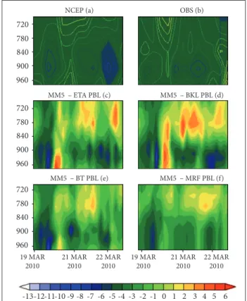
Figures 5 and 6 show the zonal and meridional components provided from the day March 19 at 12:00 UTC until the 22th at 12:00 UTC. ETA (Fig. 5c), BLK (Fig. 5d) and BT (Fig. 5e) simulations and also data from the NCEP reanalysis (Fig. 5a) underestimated the observed zonal. Only the prediction MRF (Fig. 5f) was treated in the observation of the entire length of the air layer and analyzed throughout the forecast.
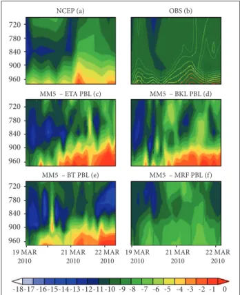
From radiosonde launches at 12:00 UTC (Fig. 6), it was noted again the permanence of negative sign of the simulated meridional component for all forecasts (Figs. 6c, 6d, 6e and 6f)
Figure 4. Example of comparisons of the meridional wind component (m/s) between 1,000 and 700 hPa. (a) Reanalyses - NCEP. (b) Radiosoundings at CLA; MM5 simulations utilizing the ETA (c), BLK (d), BT (e) and MRF (f) parametrizations.
Figure 5. Example of comparisons of the zonal wind component (m/s) between 1,000 and 700 hPa. (a) Reanalyses - NCEP. (b) Radiosoundings at CLA; MM5 simulations utilizing the ETA (c), BLK (d), BT (e) and MRF (f) parametrizations.
960 720 780 840 900
960 720 780 840 900
960
17 SEP 2008
19 SEP 2008
20 SEP 2008
17 SEP 2008
19 SEP 2008
20 SEP 2008
720 780 840 900
NCEP (a) OBS (b)
MM5 – ETA PBL (c) MM5 – BKL PBL (d)
MM5 – BT PBL (e) MM5 – MRF PBL (f)
-12-11-10 -9 -8 -7 -6 -5 -4 -3 -2 -1 0 1 2 3 4 5 6 7 8
960 720 780 840 900
960 720 780 840 900
960
19 MAR 2010
21 MAR 2010
22 MAR 2010
19 MAR 2010
21 MAR 2010
22 MAR 2010
720 780 840 900
NCEP (a) OBS (b)
MM5 – ETA PBL (c) MM5 – BKL PBL (d)
MM5 – BT PBL (e) MM5 – MRF PBL (f)
above 925 hPa, unlike the observed (Fig. 6b). Nevertheless, both are close to the value observed 24 hours ater the start of simulation from 1,000 to 850 hPa. The MRF (Fig. 6f ) simulation was a little closer observation, with only 1 – 2 m/s apart (Fig. 6b).
he graphic result of 2010 simulations showed that when the simulations were initialized at 00:00 UTC (not shown) between levels 1,000 and 925 hPa and between 700 and 850 hPa, the MRF parametrization was not surpassed by any other, that is, the prediction of zonal values obtained better results using the MRF; however, at levels between 925 and 850 hPa, the ETA, BLK, BT the parametrizations were better than the MRF, although underestimated the observed values. Whereas, when the simulations were initialized at 12:00 UTC, no parametrization was more close to the observation than the MRF parametrization, considering the whole period of 72 hours for any layer of the atmosphere studied.
According to the results obtained for the meridional component, this was not well-simulated by the PBL parameterization when initialized at 00:00 UTC (not shown)
Figure 6. Example of comparisons of the meridional wind component (m/s) between 1,000 and 700 hPa. (a) Reanalyses - NCEP. (b) Radiosoundings at CLA; MM5 simulations utilizing the ETA (c), BLK (d), BT (e) and MRF (f) parametrizations.
960 720 780 840 900
960 720 780 840 900
960
19 MAR 2010
21 MAR 2010
22 MAR 2010
19 MAR 2010
21 MAR 2010
22 MAR 2010
720 780 840 900
NCEP (a) OBS (b)
MM5 – ETA PBL (c) MM5 – BKL PBL (d)
MM5 – BT PBL (e) MM5 – MRF PBL (f)
-13-12-11-10 -9 -8 -7 -6 -5 -4 -3 -2 -1 0 1 2 3 4 5 6
and, when subjected to commence at 12:00 UTC, the ETA, BT and BLK parameterizations approached, but not exceed, the performance of MRF, which was better in 1,000 to 850 hPa layer.
VERTICAL PROFILES
Vertical Proile for the Dry Season (2008)
Figure 7 shows the forecasts with 24, 36, 48, 60 and 72 hours in advance of vertical proiles of wind speed and direction for the day September 20, 2008 from simulation initialized on September 17, 2008 at 00:00 UTC. For wind speed, the performance of the model estimates varied schedules. In some cases, the result was better forecasts for 24 and 72 hours of model integration also depending on when the simulation is initiated: 00:00 and 12:00 UTC (not shown).
he wind direction seemed to be better predicted by the model than the speed compared to observation. he parameterizations used predicted values of wind direction very close to the observations, but at certain times of the simulations with the MM5 MRF parameterization set up closer to the real value. As the wind speed, the time (integration time of the model) in which the prediction of wind direction is better was not deined. he rates difer from 1.0 to 5.0 m/s approximately, and the worst predictions of wind direction reached on average around 40 degrees of diference relative to the observed.
Vertical Proile for the Rainy Season (2010)
The vertical profiles of wind speed and direction for March 22 are shown in Fig. 8. In the same way as observed in the dry season (2008), the rainy season was not well-deined times when the predictions are better. he analysis results revealed some diferences of up to 5.0 m/s of wind intensity between the simulated and the actual value, as in the simulation for March 22, 2010 at 00:00 UTC (Fig. 8), which was well-simulated by the model considering all parameterizations, almost throughout the integration period. However, for the inal time (over 60 hours), this did not happen, mainly for ETA parameterization levels of 925 and 850 hPa. It was noted that the simulations from the MRF parameterization stood out among the others also in predicting the speed and the prediction of wind direction. An observed result is that forecasts of 24, 60 and 72 hours were better for the wind direction during the rainy season.
results show that the impact of parameterization is also not felt throughout the length of the atmosphere studied here between the levels of 700 and 1,000 hPa, that is, there are limitations in the wind forecast, in terms of u and v components; in parts of this layer, sometimes a particular parameterization performs better near the surface and, at other times, at higher levels. Basically, considering all tested options, it was noted that the model presented errors in wind velocity field mainly in 1,000 hPa. This represents that the wind field near the surface did not respond well to main features of CLA relief or suggests that we should adjust not only the parameterization of PBL, but also the physics of clouds parametrization. Considering the entire atmosphere layer studied, between 1,000 and 700 hPa, the differences were smaller in the dominant sectors of the wind, in this case, NE and SE, which somehow reduces this limitation since the most important sectors are reasonably simulated by the model.
Analysis of Concordance of Willmott Index
The impact in defining the parameterization of the MM5 PBL ideal for CLA, obtained by the wind forecast, has been reported for the dry and rainy seasons. The Willmott agreement index signaled some important results in search for the best parameterization of PBL. On average, the best results were Willmott index forecasts for 60 hours in advance, so during the dry period and for the rainy one.
Table 3 presents the comparison of the simulation results obtained for the diferent PBL parameterizations for the period from September 16, 2008 at 12:00 UTC to September 21, 2008 at 12:00 UTC for the zonal and meridional components. he best result for the Willmott index regarding the zonal component was for the MRF parametrization on both domains with values of -0.07 or fair performance for the 60-hour forecasts. he best result obtained for the meridional component of the Willmott value was -0.28 or unsatisfactory for BLK on domain 1 and -0.32 or unsatisfactory for MRF on domain 2.
Figure 7. Example of the comparison of vertical wind proiles (m/s) predicted with the ETA, BLK, BT and MRF parametrizations and the radiosounding observations (OBS) in the layer from 1,000 to 700 hPa for forecast times of 24, 36, 48, 60 and 72 hours.
OBS B–T
DIR (degree) Wind (m/s)
P
ress
ur
e (hP
a)
MRF ETA
BLK Initialisation: 00Z17SEP2008
Forecasting: 00Z18SEP2008 Initialisation: 00Z17SEP2008Forecasting: 00Z20SEP2008
720
780
840
900
960
0 4 8 12 16 20 24
720
780
840
900
960
720
780
840
900
960
720
780
840
900
960
Initialisation: 00Z17SEP2008 Forecasting: 12Z18SEP2008
720
780
840
900
960
0 4 8 12 16 20 24
Initialisation: 00Z17SEP2008 Forecasting: 00Z19SEP2008
720
780
840
900
960
0 4 8 12 16 20 24
Initialisation: 00Z17SEP2008 Forecasting: 12Z19SEP2008
720
780
840
900
960
0 4 8 12 16 20 24 0 4 8 12 16 20 24
0 100 200 300 720
780
840
900
960
0 100 200 300 720
780
840
900
960
0 100 200 300 720
780
840
900
960
Zonal component – 2008
Domain 1
Statistical index Forecast MRF BLK ETA BT
Willmott 60 -0.07 -0.08 -0.11 -0.09
Domain 2
Willmott 60 -0.07 -0.07 -0.11 -0.11
Meridional component – 2008
Domain 1
Statistical index Forecast MRF BLK ETA BT
Willmott 24 -0.31 -0.28 -0.35 -0.33
Domain 2
Willmott 24 -0.32 -0.36 -0.38 -0.36
Table 3. Statistical indices obtained for the zonal and meridional components from 1,000 to 700 hPa for the period of the dry season.
Initialisation: 00Z19MAR2010
Forecasting: 00Z20MAR2010 Initialisation: 00Z19SEP2010Forecasting: 00Z22MAR2010
720
780
840
900
960
0 4 8 12 16 20 24
720
780
840
900
960
720
780
840
900
960
720
780
840
900
960
Initialisation: 00Z19MAR2010 Forecasting: 12Z20MAR2010
720
780
840
900
960
0 4 8 12 16 20 24
Initialisation: 00Z19MAR2010 Forecasting: 00Z21MAR2010
720
780
840
900
960
0 4 8 12 16 20 24
Initialisation: 00Z19MAR2010 Forecasting: 12Z21MAR2010
720
780
840
900
960
0 4 8 12 16 20 24 0 4 8 12 16 20 24
0 100 200 300 720
780
840
900
960
0 100 200 300 720
780
840
900
960
0 100 200 300 720
780
840
900
960
0 100 200 300 0 100 200 300
DIR (degree) Wind (m/s)
P
ress
ur
e (hP
a)
OBS B–T
MRF ETA
BLK
Figure 8. Example of the comparison of vertical wind proiles (m/s) predicted with the ETA, BLK, BT and MRF
parametrizations and the radiosounding observations (OBS) in the layer from 1,000 to 700 hPa for forecast times of 24, 36, 48, 60 and 72 hours.
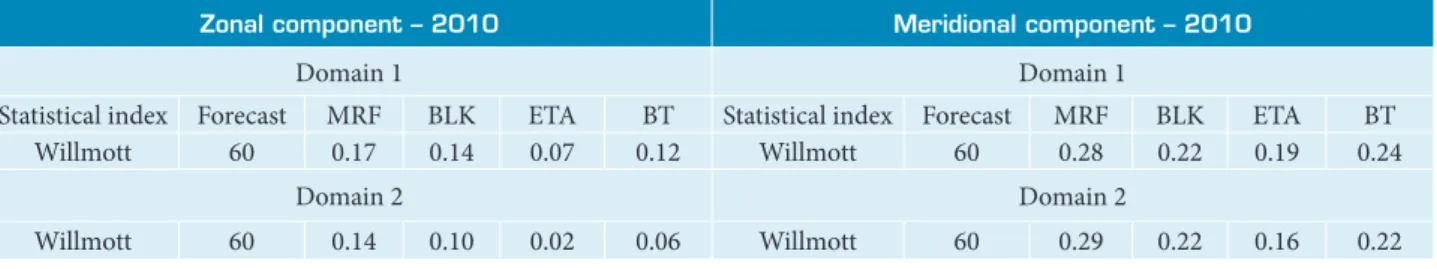
Table 4 shows results for the zonal and meridional components from the simulations initialized at 12:00 UTC for the period from March 20, 2010 at 12:00 UTC to March 25, 2010 at 12:00 UTC, in this case, wet season. he MRF parameterization did not obtain a good result; nevertheless, it was still better than the other parameterizations, both on domain 1, where it was observed the value of 0.17, as on domain 2, where it was observed the value of 0.14. hat is, for both domains, it was considered fair according to the Willmott index.
Table 4. Statistical indices obtained for the zonal and meridional components for the atmospheric layer from 1,000 to 700 hPa for the period of rainy season.
Zonal component – 2010
Domain 1
Statistical index Forecast MRF BLK ETA BT
Willmott 60 0.17 0.14 0.07 0.12
Domain 2
Willmott 60 0.14 0.10 0.02 0.06
Meridional component – 2010
Domain 1
Statistical index Forecast MRF BLK ETA BT
Willmott 60 0.28 0.22 0.19 0.24
Domain 2
Willmott 60 0.29 0.22 0.16 0.22
CONCLUSION
It was noticed in this experiment that ETA and BT parameterizations are not suitable for the CLA. Considering the available data set, in general, both default MRF and BLK parameterization presented suitable schemes. he former is better for the wet season and the latter gave the best results for the dry season. An important factor that must be emphasized is that both parameterization schemes are non-local schemes. In this case, the non-local scheme is related to vertical difusion, which is an important process that considers the efects of eddies moving to larger distances according to the physical processes that occur in turbulent atmosphere. he larger eddies are more
important as they are more sensitive to the environment. his can be the cause of the MM5 model subtly better predict the wind in PBL considering these schemes, given that non-local schemes better simulate the deep and large eddies PBLs.
It was also found that the initializations at 12:00 UTC are better than those at 00:00 UTC. Elleman et al. (2003) assert that many of the parameterizations of the boundary layer MM5, including the MRF, tend to promote an excessive vertical mixing, which means that the errors they produce are higher during the night, that is, when there is the smallest vertical mixing. Possibly overnight, the main process responsible for errors generated is the cloudiness provided, which controls the radiation of long radiation lost to space.
REFERENCES
Blackadar, A.K., 1976, “Modeling the Nocturnal Boundary Layer”. Proceedings of the 3rd Symposium on Atmospheric Turbulence, Diffusion and Air Quality, Boston, USA.
Burk, S.D. and Thompson, W.T., 1989, “A Vertically Nested Regional Numerical Weather Prediction Model with Second-Order Closure Physics”, Monthly Weather Review, Vol. 117, pp. 2305-2324.
Camillo, G.L., 2011, “Impacto das Parametrizações de Camada Limite Planetária do MM5 na Previsão de Ventos em Baixos Níveis”, Revista da Universidade da Força Aérea, Vol. 23, No. 28, pp. 67-79.
Carvalho, M.A.V., 2011, “Variabilidade da Largura e Intensidade da Zona de Convergência Intertropical Atlântica: Aspectos Observacionais e de Modelagem”, Master’s Dissertation, Instituto Nacional de Pesquisas Espaciais, São José dos Campos, Brazil.
Dudhia, J., 1989, “Numerical Study of Convection Observed during the Winter Monsoon Experiment Using a Mesoscale Two-Dimensional Model”, Journal of Atmospheric Sciences, Vol. 46, No. 20, pp. 3077-3107. doi: 10.1175/1520-0469(1989)046<3077: NSOCOD>2.0.CO;2
Dudhia, J., Gill, D., Guo, Y., Manning, K., Wang, W., and Chiszar, J., 2003, “Mesoscale Modeling System Tutorial Class Notes and User’s Guide: MM5 Modeling System Version 3”, PSU/NCAR.
Elleman, R.A., Covert, D.S. and Mass, C.F., 2003, “Comparison of ACM and MRF Boundary Layer Parameterizations in MM5”, Proceedings of the Models-3 Workshop, Raleigh, USA.
Grell, G.A., 1993, “Prognostic Evaluation of Assumptions Used by Cumulus Parameterizations”, Monthly Weather Review, Vol. 121, pp. 764-787. doi: 10.1175/1520-0493(1993)121<0764:PEOAUB>2.0.CO;2
Grell, G.A., Dudhia, J., and Stauffer, D.R., 1994, “A Description of the Fifth-Generation Penn State/NCAR Mesoscale Model (MM5)”, NCAR Technical Note, NCAR/TN-398+STR, Boulder, USA, 117 p.
Hong, S.-Y. and Pan, H.-L., 1996, “Nonlocal Boundary Layer Vertical Diffusion in a Medium-Range Forecast Model”, Monthly Weather Review, Vol. 124, No. 10, pp. 2322-2339. doi: 10.1175/1520-0493(1996)124<2322:NBLVDI>2.0.CO;2
Janjic, Z., 1994, “The Step-Mountain Eta Coordinate Model: Further Developments of the Convection, Viscous Sublayer, and Turbulence Closure Schemes”, Monthly Weather Review, Vol. 122, No. 5, pp. 927-945. doi: 10.1175/1520-0493(1994)122<0927:TSMECM>2.0.CO;2
Johnson, D.L., 2008, “Terrestrial Environment (Climatic) Criteria Guidelines for Use in Aerospace Vehicle Development, 2008 Revision”, NASA/TM 2008-215633, Marshall Space Flight Center, Alabama, USA.
Mellor, G.L. and Yamada, T., 1974, “A Hierarchy of Turbulence Closure Models for Planetary Boundary Layers”, Journal of Atmospheric Sciences, Vol. 31, No. 7, pp. 1791-1806.
Oyama, M.D. and Giarolla, E., 2006, “Simulação de Linhas de Instabilidade na Costa Norte do Brasil de 6 a 9 de Julho de 2005 com o Uso do Modelo Regional MM5: Resultados Preliminares”, Proceedings of the XIV Brazilian Congress of Meteorology, Florianópolis, Brazil.
Pereira Neto, A.V. and Oyama, M.D., 2011, “Mudanças do Esquema de Convecção Profunda Kain-Fritsch para a Região do Centro de Lançamento de Alcântara”, Revista Brasileira de Meteorologia, Vol. 26, p. 579-590.
Willmott, C.J., Robeson, S.M. and Matsuura, K., 2011, “A Reined Index of Model Performance”, International Journal of Climatology,
Vol. 32, No. 13, pp. 2088-2094. doi: 10.1002/joc.2419
Wyngaard, J.C. and Brost, R.A., 1984, “Top-Down and Bottom-Up Diffusion of a Scalar in the Convective Boundary Layer”, Journal of Atmospheric Sciences, Vol. 41, p. 102-112. doi: 10.1175/1520-0469(1984)041<0102:TDABUD>2.0.CO;2