ABSTRACT: A turbulent reacting low in a channel with an obstacle was simulated computationally with large eddy simulation turbulence modeling and the Xi turbulent combustion model for premixed lame. The numerical model was implemented in the open source software OpenFoam. Both inert low and reactive low simulations were performed. In the inert low, comparisons with velocity proile and recirculation vortex zone were performed as well as an analysis of the energy spectrum obtained numerically. The simulation with reacting low considered a pre-mixture of propane (C3H8)
and air such that the equivalence ratio was equal to 0.65, with a theoretical adiabatic lame temperature of 1,800 K. The computational results were compared to experimental ones available in the literature. The equivalence ratio, inlet low velocity, pressure, lame-holder shape and size, fuel type and turbulence intensity were taken from an experimental set up. The results shown in the present simulations are in good agreement with the experimental data.
KEYWORDS: Computational luid dynamics, Reacting low, Large eddy simulation, Combustion modeling.
Large Eddy Simulation of Bluff Body Stabilized
Turbulent Premixed Flame
Nicolas Moisés Cruz Salvador1, Márcio Teixeira de Mendonça2, Wladimyr Mattos da Costa Dourado2
INTRODUCTION
In turbulent reactive low simulations, computational models have achieved a great development in recent years with the improvement of computer power. his development allowed more accurate solution of problems such as the instability caused by the turbulence in combustion chambers of rocket engines, gas turbines, turbojet aterburners, ramjets and scramjets. hese models have been used to study bluf body stabilized lames, which allow combustion devices to operate at very high free stream velocities. Advanced aterburner design methods have been discussed by Lovett et al. (2004), who outlined the fundamental combustion sciences and engineering challenges that need to be addressed. Among other problems, Lovett et al. (2004) highlighted the requirements for lame stabilization and combustion dynamics. hese authors discuss the need for advanced design methodologies and tools, and they stress the limitations of existing computational models to capture the physics of those phenomena.
In turbulent combustion, the behavior of the turbulent lame front is predominantly dictated by the turbulence (Peters, 2000). Combustion instability is also directly related to turbulence (Weller, Marooney and Gosman, 1990). herefore, it becomes mandatory in numerical simulations to use turbulence models that reproduce these dynamic processes, which are mainly produced by large scale turbulence. Many researchers have used Reynolds Averaged Navier Stokes (RANS) and eddy viscosity turbulence models to simulate reactive lows behind bluf bodies. However, important discrepancies were observed due to shortcomings in the RANS methodology, especially in complex lows with circular obstacle (Saghaian et al.,
1.Instituto Nacional de Pesquisas Espaciais – São José dos Campos/SP – Brazil 2.Instituto de Aeronáutica e Espaço – São José dos Campos/SP – Brazil Author for correspondence: Marcio Teixeira de Mendonça | Instituto de Aeronáutica e Espaço | Praça Marechal Eduardo Gomes, 50 – Vila das Acácias | CEP 12.228-904 São José dos Campos/SP – Brazil | E-mail: [email protected]
2003; Frendi, Skarath and Tosh, 2004) and triangular one (Bai and Fuchs, 1994; Dourado, 2003; Eriksson, 2007). Signiicant diferences in results were found for the turbulent velocity, integral length scale and turbulent viscosity distribution between RANS models. hese diferences afect the computation of lame front difusion, which is under-predicted. he Kelvin-Helmholtz efects behind the obstacle are not captured well and the length of the recirculation zone as well as the turbulent lame speed are not recovered.
Experimental studies were conducted by Sjunesson, Henriksson and Lofstrom (1992) and Sjunnesson, Olovsson and Sjoblom (1991) at Volvo (Sweden). he Volvo test rig had an equilateral triangular bluf body with a blockage of 33% and a Reynolds number (Re) based on the inlet velocity and two times the channel height of 204,000. For this Re, the Strouhal number (St) observed was 0.417. he premixed gases were air and propane at equivalence ratios of 0.65 and 0.85. he Damköhler number (Da) was 10 and the Karlovitz number (Ka) was 4. he resulting lame for these conditions was on the thickened-wrinkled lame regime of the Borghi diagram rather than in the wrinkled lame regime. Sanquer (1998) also presented experimental results for premixed lame stabilized by a triangular prismatic bluf body at the University of Poitier (France). he blockage in his experiments was also 33% for a Re in the range of 6,690 to 23,150, much lower than the Re on the Volvo experiments. he St for the lower Re experiment was 0.276. herefore, the vortex shedding characteristics and the turbulent scales (integral and Kolmogorov) were signiicantly diferent from the Volvo experiment. Sanquer’s results will be discussed and compared to the present numerical simulations on the following sections. Speciically, the present simulations correspond to Sanquer’s experiment that falls on the Borghi diagram where Da<1 and Ka>1 corresponding to the thin-wrinkled lame region.
hese and other experimental results (Cheng, 1984, Cheng, Shepherd and Gokalp, 1989, Cheng and Shepherd, 1991, Kiel et al., 2007, Chaudhuri et al., 2011) describe the interaction between the turbulent structures and the lame. Numerical simulations of turbulent combustion must rely on models that are able to capture the complex turbulent vortical structures and this explains why results obtained with RANS models are less accurate. In order to improve numerical simulations, turbulent combustion models can be ported from RANS models to Large Eddy Simulation (LES) models, which are known to capture the large scale turbulent structures. his approach does not always result in more accurate
simulations. It is necessary to identify those models that have the best results and show greater potential for future improvements when used in LES.
A number of investigators have used LES to simulate reactive lows with bluf body lame holders. Porumbel and Menon (2006), Akula, Sadiki, and Janicka (2006), Ge et al. (2007), Park and Ko (2011) and Manickam et al. (2012) simulated the Volvo experiment (Sjunnesson, Olovsson and Sjoblom, 1991). Porumbel and Menon (2006) have simulated bluf body lows with the Linear Eddy Mixing (LEM) LES based on the model proposed by Kerstein (1989) and developed into a sub-grid model by Menon et al. (1993) for premixed combustion. hey discussed the diferences between their model and the Eddy Breakup model (LES-EBU) and which of the two is best to represent the physics of the reacting low behind an obstacle besides the ability to resolve the turbulent eddies that wrinkle the lame front. his model is specially adequate for high turbulent intensities where the chemical time is considered ininitely small, corresponding to a Da much greater than 1. heir conclusions were conirmed by experimental results presented by Chaudhuri et al. (2011).
Akula, Sadiki, and Janicka (2006) also performed LES simulations with a lame surface density formulation adapted from Boger and Veynante (2000). his model includes the resolved progress variable in the transport equations and the lame wrinkling model avoids unrealistic detachment of the lame from the lame holder. he compressible model presented by Tabor and Weller (2004), along with a similar progress variable approach, is also able to capture the lame wrinkling and thus capture the physics as proposed by Porumbel and Menon (2006). he model of Tabor and Weller (2004) is used in the present simulations.
behind the obstacle due to combustion. he results for the dynamic model show better agreement with experimental results when compared with the Smagorinsky model. he unsteady low ield was captured with good accuracy and the temperature and reaction rate proiles are well capture by both models, showing that the two combustion models tested are reasonable for the simulation of pre-mixed combustion behind a bluf body.
Manickam et al. (2012) used an algebraic lame surface wrinkling (AFSW) reaction model based on the progress variable approach. Inert and reacting cases were analysed and compared with experimental results and with another well validated turbulent lame speed closure model denominated Turbulent Flame Speed Closure (TFC) (Zimont and Lipatnikov, 1995). For the non-reacting test case, they found a shedding frequency equal to 122Hz, while the experimental measured frequency was 110Hz. he comparisons for the mean low variables and root mean square axial and normal velocity components were in good agreement with the experiments. In spite the fact that the recirculation zone length was well captured, the rms velocity distributions were underpredicted in this zone. Manickam et al. (2012) presented a detailed discussion on the inluence of grid reinement and three subgrid scale models on the results and concluded that a coarse grid is too dissipative. Contrary to what might be expected, the grid reinement has a weak inluence on the computation of the St, showing that at least the large scale structures were captured by a course grid LES simulation. he St dependence on the grid was also not observed for the reactive case, independently of the reaction model. he three sub-grid scale models tested were the Smagorinsky (SM), the dynamic Smagorinsky (DS) and the sub-grid scale kinetic energy (KSGS). hey showed that the performances of the three diferent models are more or less equivalent.
Flame Surface Density (FSD) models rely on geometric parameters of the lame front to evaluate its progress. In this case, the laminar lamelet model used in RANS has been adapted to LES by considering a locally laminar lame wrinkled by turbulence. he amount of wrinkling (Σ) is measured by the lame surface area per unit volume (Boger and Veynante, 2000). Transport equations for the progress variable and for the wrinkling variable are solved to describe the evolution of the lame since the wrinkling increases the burning rate.
Similar to the Σ variable, Weller (1993) proposed a model based on the density of wrinkling (Ξ), which is the lame
area per unit area resolved in the mean direction of propagation. Weller (1993) originally developed this model for RANS and later Tabor and Weller (2004) adapted the model for LES. he advantage of using Ξ is that it should be easier to model the transport terms as discussed in Weller (1993), Weller et al. (1998) and Tabor and Weller (2004). his model is used in the present study and will be discussed in detail on the following sections.
In the present study, the SM and dynamic sub-grid models for turbulence were used. For the combustion model, the lame surface wrinkling (Ξ) formulation, developed by Tabor and Weller (2004), was used. he objective of the study was to investigate the performance of a turbulent combustion model when applied to the simulation of pre-mixed turbulent lames behind a triangular obstacle. he review of the literature shows that such type of performance investigation has been conducted previously, with results compared to the Volvo experiment, which has a Dain the range of 10 and a Ka of 4, corresponding to a thickened, wrinkle lame. he present investigation considered an experiment which has a Da of 4.5 and a Ka of 1.3; on the range of thin, wrinkled lame, previous investigations found in the open literature did not consider LES simulations in this combustion regime, and the thinner lame thickness poses a more severe test for the turbulent combustion model. he Re for the simulation was 6,690, lower than the Re on the Volvo experiment, which was 204,000 and thus have a signiicant diferent low dynamics. he chosen reactive LES model was evaluated by comparing results with experimental ones obtained by Sanquer (1998), which have not been analyzed before with other LES numerical models.
PROBLEM FORMULATION
In order to account for turbulence and combustion, the reactive low governing equations are iltered using the LES concept, and the combustion process is accounted for by following the lame front. herefore, it is necessary to deine the iltering and a variable to account for the regions of burned and unburned gases. In this section, the formulation derived by Weller (1993) and Tabor and Weller (2004) is presented.
PRELIMINARY DEFINITIONS
this propagation, varies between 0 for fresh gas and 1 for burned gas. he transitions between these values describe the lame front. A progress variable c can be deined based on the normalized temperature (T) or on the reactant mass fraction (Y). Using the temperature, it results in:
u b
u T T
T T c
− −
= . (1)
Where b subscript stands for burned gas and u subscript, for fresh unburned gas. he lame front propagation is modelled by solving a transport equation for the density-weighted mean reaction regress variable denoted by b , where b =1 - c.
In LES, it is assumed that the dependent variables can be divided into grid scale (GS) and sub-grid scale (SGS) components, such that, for any given dependent variable, it results in:
ψ
ψ
ψ
=
+
ʹ
.
(2)Where
. t ) d
,
Δ ) ψ (
,
(
G ψ * G
ψ 3
D
x' x' x'
∫
= (3)
Here, D is the computational domain with boundaries ∂D , t is the time and x, the coordinate directions. he kernel
G = G (x,∆) is any function of x and of the ilter width ∆. G has the properties ∫D G(x)d3x=1, lim
∆→0 G(x,∆)=δ(x)
Introducing a conditional ilter (Tabor and Weller, 2004), with an indicator function l, results in:
0
) , ( if 1 ) , (
⎩ ⎨ ⎧
= t
t
l x x (4)
is in the unburned gas region otherwise.
For a tensor ψ of any rank, one may deine ψ the phase-= ʹ ʹ ʹ ʹ weighted value of ψ at any point.
x x x x
x− ʹ ʹ ʹ ʹ
=
=
∫
3) , ( ) , ( ) ( ) (
* l G l t td
G
D
ψ ψ
ψ . (5)
Introducing the combustion progress variable b as a GS indicator function, we can obtain:
, u
bψ
ψ = (6)
where b(x , t ) is the probability of the point (x , t ) being in the unburned gas.
. x x x
x− ʹ ʹ ʹ
=
∫
3D
t)d , )l( ( G
b (7)
In compressible low, there is density (ρ) variation, and the product ρψ = can be written:
b ρψ
ρψ = . . (8)
Where the subscript u indicates the unburned gases.
Deining a density-weight average ψu ~
in the unburned phase, we can obtain:
u
u ρψ
ρψ = ~ . (9)
From Eq. 8 in Eq. 9, results in:
. ~
u
bρψ
ρψ = (10)
FILTERED CONTINUITY EQUATION
he governing equations will be written in a coordinate system placed at the lame surface, such that n⊥ and n|| are the unity vectors pointing the normal x⊥ and parallel x|| directions to the lame surface. he metrics of this coordinate system are
h⊥ and h||. his coordinate system is used in order to include the conditional ilter based on the progress variable b.
he iltered continuity equation reads (Tabor and Weller, 2004):
. ) ( − ⋅ Σ =
⋅ ∇ + ∂ ∂
⊥
n U U
U ρ I
ρ ρ
t . (11)
Where UI=U+van⊥ ,UI is the full velocity on an interface consisting of the movement due to advection term U=U+ and the ⊥ advance of the interface relative to the low = +van⊥.,
In the transformed coordinates for (x⊥,x||):
. | | ) ( )
( 2
|| || ||
, G x x d x||
x x G
I − ʹ ℑ
− =
W h e re |ℑ represents the Jacobian of the transformatio| ʹ n. | | 2 || x d
ℑ ʹ is the area element on the surface interface. Σ is interpreted as the amount of interface for the iltered component, the lame surface density.
he surface iltering operation ⎩ ⎨ ⎧ is deined as:
∫
− ʹ ʹ ʹ− ⋅ ʹΣ = ⊥ ⊥ D d h
G x x x x x n 1 3x
) ) (( ) ( ) ( 1
ψ ψ δ . (13)
From Eq. 10 in Eq. 11, results in:
. v ~ aΣ − = ⋅ ∇ + ∂
∂ ρ ρ ρ
u u
u b
t b
U . (14)
his surface iltering operation applied to
n
⊥ results in:
∫∫
− ℑ ʹ− Σ = ⊥ ⊥ ⊥ ⊥ ⊥ ⊥ || 2 || | , || || || ,) ( ' ) ( , ')| | ( 1 x n x x d x x G x x G
n I I . (15).
ʹ =
⊥ 1
n can be related to the GS with the n
fdirection of the interface: Ξ = ⊥ f n
n . (16)
Where Ξ represents the total sub-grid surface area by the smoothed surface area in the
n
f direction: | ( ) ( ') ( , ' )| | |. 1 || 2 || , || || ||
,
∫∫
− ℑ ʹ− Σ = = Ξ ⊥ ⊥ ⊥ ⊥ ⊥ ⊥ x n
n G x x I G x x x I x d
.
(17)
Or:
|
|∇b
Σ =
Ξ . (18)
Where |∇b|
=
represents the area of the GS surface.
Combining the burned and unburned gases into the weighted total density results in:
) (1 b b c
u + −
=ρ ρ
ρ . (19)
Such that ρb~=ρub. .
he inal continuity equation reads:
| | ) ~ ~ ( ~ b S b t b u u u =− Ξ ∇ ⋅ ∇ + ∂ ∂ ρ ρ ρ
U , (20)
where Su is the laminar lame speed.
FILTERED MOMENTUM AND ENERGY EQUATIONS
Conditionally iltering the momentum equation gives:
{
}
Σ⎥ ⎥ ⎦ ⎤ ⎢ ⎢ ⎣ ⎡ − ⋅ − + − ⋅ +∇ −∇ = ⊗ ⋅ ∇ + ∂ ∂ ⊥ ) ( ( ) ( ) ~ ~ ( ~ U v n S ) I B U U U a ρ ρ ρ p S b p b b t b u u u u u u u u (21) .
Where p is the pressure, Su is the laminar lame speed, Σ is the lame surface density, S=λ∇⋅UI+2μ is the stress
tensor and ( )
2
1 T
U U+∇ ∇
= is the symmetric part of the strain tensor. he terms in brackets represent the efect of the interface on the momentum balance.
B
urepresents the SGS stress tensor.
u u u
u U U
U U Bu ~ ~ ) ( ⊗ − ⊗
= ρ ρ . (22)
his term requires modeling.
he iltered energy equation is:
. ) ( ) ( ) ( ) ~ ( ) ~ ~ ( ) ~ ( Σ ⎥ ⎥ ⎦ ⎤ ⎢ ⎢ ⎣ ⎡ ⋅ − + − ⋅ ∇ + + ⋅ + + ⋅ ∇ − = ⋅ ∇ + ∂ ∂ ⊥ n h v b h D S U a u u u u e b b b b U b e b t e b u u u u u u u u u u u ρ ε ρ π ρ ρ ρ ρ (23) Where , ~ )
(∇⋅U + ∇⋅Uu
= u u
u
uπ p p
ρ , (24)
and
, )
( u u
u
uε = S⋅D +SuD
represent the SGS pressure dilatation π and dissipation ρuεu= ⋅ + (Tabor and Weller, 2004). he total energy at the interface is
presented in brackets.
TURBULENCE MODEL
In the present study, three turbulence models available in OpenFoam were used. hese turbulence models are described by Fureby et al. (1997). First, the Smagorinsky classical model is presented: ) ~ 3 ~ ( 2 ~ 3 2 ~ ~ 3 kk ij ij sgs k k ij i j j i t kk ij ij S S x u x u x u δ υ ρ δ ρ υ τ δ τ − − = ⎟ ⎟ ⎠ ⎞ ⎜ ⎜ ⎝ ⎛ ∂ ∂ − ∂ ∂ + ∂ ∂ − = − . (26)
Where υsgs is the sub-grid viscocity and ( ⎟⎟ ⎠ ⎞ ⎜ ⎜ ⎝ ⎛ ∂ ∂ + ∂ ∂ = i j j i ij x u x u S ~ ~ 2 1 ~
is the strain tensor.
S Cs 2 sgs
~ )
( Δ
=
υ . . (27)
he constant Cs is equal to 0.18.
he second turbulence model is the one-equation model with sub-grid kinetic energy k~ proposed by Yoshizawa and = Horiuti (1985) and given by:
(
k k k k)
kk uu uu
k ~~
2 1 2 1 ~ − =
= ρτ . . (28)
where the operation
a
stands fora
~
in the productu
ku
k above.he sub-ilter stress is:
ij kk ij ij v ij k 3 2 S 3 S k C
2ρ δ ρ δ
τ ⎟⎟+
⎠ ⎞ ⎜⎜ ⎝ ⎛ − Δ −
= ~ ~ , (29)
and turbulent viscosity is: vsgs =ρC kΔ k .
To close the system of equations, the transport equation for the kinetic energy is used.
ε ρ ρ − − = ∂ ∇ ∂ − ∂ ∂ + ∂ ∂ B u k v u k u t k i k i i : ~
D . (30)
where Δ = 3 /2 e k C ρ ε
, (31)
and dev(D) 2v kI 3 2
B= − k . (32)
he third turbulence model is the dynamic one-equation model that used the Germano identity, following Ghosal et al. 1995, considering a scaling law and homogeneous low. he kinetic energy equation is:
ε ρ ρ − − = ∂ ∇ ∂ − ∂ ∂ + ∂ ∂ B L u k v u k u t k i k i i ~ , (33)
where L is the Germano identity (Ghosal et al., 1995): B
T
L= − with:
) ( ), ( ), ( u u u u B u u u u T u u u u L ⊗ − ⊗ = ⊗ − ⊗ = ⊗ − ⊗ = . (34)
SUBGRID COMBUSTION MODEL
Models for the SGS stress tensor, lux vectors, dissipation and iltered reaction rates are used to close the governing equations. he models for the SGS stress tensor and lux vectors are the standard ones used in LES, since they do not depend on reacting low data.
A lamelet model with conditional iltering for LES is used to derive the transport equations. his model considers conditions of the Klimov-Williams criterion (Ka=1) in the Borghi diagram (Borghi and Destriau, 1998). Instead of using the lame propagation speed in terms of the laminar lame area per unit volume Σ and the degree of wrinkling of the lame at a point in the domain, the present model (Weller, 1993) uses the lame surface density and a wrinkling surface function Ξ. he function Ξ is the average lame area per unit volume divided by the projected area in the mean direction of propagation.
of the reaction zone is needed. In other words, equations for the geometric variables b and Ξ are needed.
Sub-grid scale model for b
In Eq. 20, the right hand side needs a SGS model, which is based on the conditional ilter of unburned gas velocity Uu
~ = . his term is modeled using:
uc u U 1 b U
U~ = ~+( −~)~ . (35)
where U~uc= is the slip velocity of the unburned minus burned
gas U~uc=U~u−U~c . .
his is similar to the properties of laminar lame for LES:
) ~ ( ~ ~ ) ( ~ b 1 b b S 1 U u c u uc − ∇ − Ξ − = D f n ρ
ρ , (36)
where is the difusion coeicient of the sub-grid, and | | / b b ∇ ∇ = f
n is the lame normal direction.
From Eq. 20, one arrives at the inal equation for b (Tabor and Weller, 2004):
.| | ) ~ ( ) ~ ~ ( ~ b S b b U t b u u Ξ ∇
− = ∇ ⋅ ∇ − ⋅ ∇ + ∂
∂ρ ρ ρD ρ . (37)
Sub-grid scale modeled equation for Ξ
From the transport equation for the sub-grid flame area density Σ, proposed by Weller (1993), an equation for Ξ is obtained from the relation Ξ=Σ/|∇b| and the resolved unburned gas volume fraction b (Tabor and Weller, 2004):
Ξ ∇ ∇ ∇ ⋅ − + ⋅ ∇ ⋅ Ξ + ⋅ ∇ ⋅ Ξ − = Ξ ∇ ⋅ + ∂ Ξ ∂ ⊥ ⊥ | | | | ( b b ) t I t f t f I U U n U n n U n U . (38) where − +( t U
is the surface-iltered efective velocity of the la- me and
−UI)
is the local instantaneous velocity of lame surface.
he proposed model for Eq. 38 considers wrinkling generation =GΞ− and removal −R (Ξ −1)+, such that (Tabor and Weller, 2004):
[
]
) max(σ σ ),0 Ξ
1 (Ξ R GΞ Ξ U t Ξ t s
s ⋅∇ = − − + −
+ ∂
∂ , (39)
|| ||
T
t t U
U +∇ ∇ = 2 1 t σ ⎧ ⎨ ⎩ ⎩⎨ ⎧ , (40) and || || 2 1 T I I U
U +∇ ∇ = s
σ . (41)
he models for G and R, which accounts for the interaction between turbulence and lame, are:
eq eq Ξ Ξ R
G = −1 , (42)
and ∗ ∗ − = e q e q η Ξ Ξ τ
0 .2 8
R 1 , (43)
where η u eq Re S u
0. 6 2 1
Ξ∗ = + ʹ , (44)
1). )(Ξ b 2(1 1
Ξeq= + − eq−
∗
. (45)
where Re
τ
η ʹis the Kolmogorov time, u´ is the intensity of turbulence in the sub-grid and η
u
Re S
uʹ , is the Kolmogorov
Reynolds number.
Finally, an equation for the laminar flame speed (Tabor and Weller, 2004) is needed. A proposed transport equation is: . ) ( ) ( 0 0 ∞ ∞ − − + − = ∇ ⋅ + ∂ ∂ u u u u u s u s u u S S S S S S S t S σ σ
Us . (46)
The convective velocity of the laminar flame is the filtered surface speed
∞ ∞ − − + − = ∇ ⋅ + ∂ ∂
NUMERICAL MODEL
h e present investigation uses OpenFoam, an open source C++ collection of libraries for transport equations. h e model equations are solved numerically based on a cell centered unstructured i nite volume scheme. h e solution is based on a segregated approach. For time integration, a i rst order explicit Euler method is used. For spatial discretization, second and third order Total Variation Diminishing (TVD) schemes are used. h e PISO algorithm (pressure-implicit split-operator) is used to solve the pressure-velocity coupling. h e discretization method is the standard Gauss i nite volume integration. h e combustion solver called Xifoam, available on OpenFoam, was used. h is premixed turbulent combustion model is described in the previous section – Preliminary dei nitions (Weller et al., 1998; Tabor and Weller, 2004).
Both reactive and non-reactive cases were run on a SGI Altix XE 1300 cluster with Intel x86 64 processors, running SUSE Linux Enterprise Server version 10. The cluster has 144 cores with 432 GB, DDR3, 1066 MHz RAM. For the non-reactive cases running with 64 cores, the average seconds per iteration computational time for a simulation using SM was 1.47 seconds. The clock time was about 12h52m. For the reactive case running with 136 cores, the average seconds per iteration for a simulation using the dynamic model was 8.04 seconds.
INITIAL AND BOUNDARY CONDITIONS
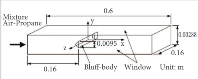
h e geometry of the channel with a bluf body l ame holder is presented in Fig. 1. It consists of a channel 0.600 m long, 0.160 m wide and 0.0288 m tall. h eRe based on the inlet velocity and twice the channel height (Re=Uaxe2h/ν) is 6,690. h e obstacle used as l ame holder is an equilateral triangular cross section obstacle whose backside is located 0.160 m from the entrance. h e obstacle blockage is 33% of the total area and corresponds to the r-65 test case in Sanquer’s experiment (Sanquer, 1998).
First, only inert simulations are considered with an initial temperature of 300K. At the outl ow boundary, a pressure wave transmissivity boundary condition is used for pressure (Candel, 1992). A uniform velocity proi le is imposed at the entrance with a speed of Uaxe=3.1 m/s to match the experimental value. On top of the uniform average velocity proi le at the inlet, a l uctuation is added using a
routine available on OpenFoam that mimics the turbulent statistical properties. h is procedure is necessary since the inlet turbulence determines the l ow behavior on the domain, as discussed by Tabor and Baba-Ahmadi (2010).
h e l ow is considered periodic in the spanwise direction. A wall function is used in the channel walls, as shown schematically in Fig. 2 (Jayatilleke, 1969).
For reacting l ows, propane (C3H8) premixed with air is considered. h e mixture is ignited behind the obstacle in the recirculation zone to achieve a proper performance and avoid l ame blow of . h e ignition point is located at 0.05m behind the obstacle in the center of the recirculation zone. A combustion time of 3ms was used before collecting data to avoid numerical transients and allow time to achieve stable combustion behavior. h e imposed initial l ame speed was 0.256 m/s and the initial condition for the regress variable was b=1.
I m p o s e v e l o c i t y p r o fi l e
W a l l
W a l l c h a n n e l
W a l l f u n c t i o n O b s t a c l e
H
=
2h
d
Exit conditions
Figure 2. Schematic boundary conditions. Turbulent velocity proi le at the channel entrance, walls and obstacle.
Figure 3. Grid structure around the obstacle.
Figure 1. Scheme of Sanquer’s experiment.
M i x t u r e A i r - P r o p a n e
0. 16
0
0. 6
0. 0095 y
x z
0. 16 0. 00288
h e grid used in the present study is composed of 388,355 volumes for two-dimensional simulations and 2,300,000 volumes for three-dimensional simulations. Figure 3 shows the grid topology around the obstacle. Lower grid densities were tested but it was not possible to reco-ver the recirculation zone size obtained by Sanquer (1998). h e adequacy of the grid was also tested through the turbulent decay rate, which should follow the Kolmogorov -5/3 decay, as discussed in the next section.
A detailed study of grid requirement using grid quality assessment techniques was presented by Manickam et al. (2012). h ey simulated the Volvo experiment using LES and a l ame surface wrinkling reaction model based on the progress variable, similar to the model used in this investigation. h eir i nest grid size has 2.4 million cells, close to the grid size used in the present investigation. h eir intermediate and i ne grids were able to recover all relevant experimental results for mean and turbulent quantities as well as the St. Nevertheless, even the i ne grid presented lower quality near the l amelet region. Considering that the Volvo experiment has a Re much larger than the Sanquer’s experiment, it is safe to say that the i ne grid for the Volvo higher Re should capture all the relevant structures for the Sanquer’s lower Re experiment and will allow the necessary level of accuracy for the sub-grid scale model.
h e instantaneous velocity was monitored in order to establish the time for which the l ow can be considered periodic stationary. Figure 4 shows the history of longitudinal velocity. As can be seen, the transition lasts 0.18 seconds, so the l ow can be considered periodic stationary beyond that.
RESULTS
In this section, the performance of the turbulent combustion models presented in problem formulation section and available on OpenFoam is assessed for the l ow conditions considered by Sanquer (1998).
First, results are presented in terms of frequencies fq and Strouhal numbers (St=fqd/Uaxe) of the vortex emission frequency behind the obstacle, where d is the obstacle height and Uaxe is the maxim velocity at the channel entrance. h e size of the average recirculation zone Xr is also compared. Next, the energy spectrum is analysed in order to verify the adequacy of the computational grid and
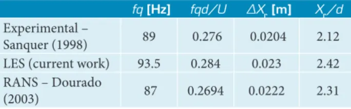
Table 1. Comparison of numerical Large Eddy Simulation (LES) and Reynolds Averaged Navier Stokes (RANS) results with experimental results.
fq [Hz] fqd/U ∆Xr[m] Xr/d
Experimental –
Sanquer (1998) 89 0.276 0.0204 2.12
LES (current work) 93.5 0.284 0.023 2.42
RANS – Dourado
(2003) 87 0.2694 0.0222 2.31
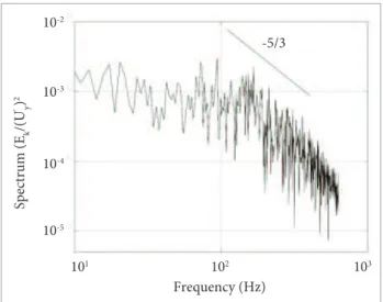
to compare the inertial range against the -5/3 turbulence decay rate for both inert and reactive cases (Pope, 2000). h en, streamwise and normal velocity proi les are compared to the experimental results in the recirculation zone and downstream of the recirculation zone. Finally, the progress variable and temperature proi les are presented.
h e recirculation zone and the energy spectra are determined through the velocity data at er the simulation reaches the stationary periodic state. Once the length of the recirculation zone Xr is determined, one can calculate the St to compare it with experimental results. To determine the values of the energy spectrum, the Fast Fourier Transform (FFT) of the oscillatory instantaneous velocity is taken. h is information is used to determine if the simulation captures the large turbulent scales and models the sub-grid scales correctly.
INERT FLOW CASE
First, inert l ow results are presented. Table 1 presents the frequencies, St and recirculation zone length for the present
t(s) 6.5
6 5.5 5 4.5 4 3.5 3 2.5 2 1.5 1 0.5 0
0 0.05 0.1 0.15 0.2 0.25 0.3 0.35 0.4
Ux(m/s)
LES simulation and for RANS simulations performed by Dourado (2003). h e results show good agreement with those obtained experimentally.
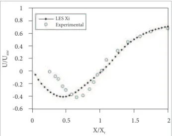
h e length of the recirculation zone based on the evolution of the average velocity Ux was determined taking the average values along the X axis downstream of the obstacle. Figure 5 shows the proi le of the average velocity used to dei ne the recirculation zone as shown schematically in Fig. 6. h e length of the recirculation zone found in the present simulation is 0.023m, while the length found by Sanquer (1998) is 0.0204m, and a simulation based on a RANS model (Dourado, 2003) gives 0.0222m. h e recirculation zone length dif ers approximately 11.5% from the experimental value.
To determine the vortex emission frequency, a temporal Fourier analysis was used (Dourado, 2003). For the numerical simulation using LES, a value of 93.5Hz was found, as shown in Fig. 7, while the experimental result was fq = 89Hz. h ese values correspond to a St=0.284 for the simulation and St=0.276 from the experiment with a dif erence of only 3%. h e RANS model gives fq=87 Hz and St=0.2694, with 2.39% dif erence in the St to the experimental result in this inert case.
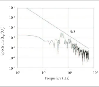
For the three-dimensional simulations, the energy spectrum shown in Figs. 8 through 11 has the -5/3 energy decay rate expected for large Re turbulent l ows. Figures 8 and 9 are the spectrum for the streamwise velocity component at X/Xr=1.4, in two dif erent distances from the channel centerline, y/h=0.1 and y/h=0.41, respectively. Figures 10 and 11 are spectrum at those two same positions, but for the normal velocity component. On the energy spectrum in Figs. 9 and 11, peaks at about 80Hz can be identii ed. h ese peaks correspond to the large scale vortex shedding frequency measured above the channel centerline. At the centerline on Figs. 8 and 10, the peaks seem to be at 100Hz but the spectrum is not conclusive.
Filtered longitudinal Ux and normal Uy component velocity proi les at X/Xr=0.8 and X/Xr=1.4 are shown in Figs. 12 to 15. Figure 12 shows the longitudinal velocity proi les in the normal direction obtained in the simulation at X/Xr=0.8. h e results are in good agreement with the experimental results, but the dynamic model overpredicts the velocities in the region behind the obstacle and does not show the reverse l ow in the recirculation zone. Downstream of the recirculation zone at X/Xr=1.4 (Fig. 13), the longitudinal velocity distributions are also close to the experimental results, even for the dynamic model, which now shows
a moderate underprediction. h e results obtained with the SM and one equation models are more accurate.
h e normal velocity component is underpredicted by all models in the regions behind the obstacle (y/h<0.6; Fig. 14), with the dynamic model showing the worse results. Approaching the upper wall (y/h greater than 0.6) the turbulence models give better predictions, but the Smagorinsky model gives results a little higher than the experiments. Never the less, the results are within the limits of the experimental error.
U axe
Xm
<u>
0
X Xr
-Ur
Figure 6. Schematic representation of the velocity distribution (Sanquer, 1998).
1
0.8
0.6
-0.6 0.4
-0.4 0.2
-0.2 0
0
X /X r
LES Xi Experimental
U/U
axe
0.5 1 1.5 2
Spectrum (E
k
/(U
')y
2
Frequency (Hz) -5/3
10-5 10-4 10-3 10-2 10-1 100 101 102
100 101 102 103
Figure 10. Energy spectrum of the normal velocity components Uy at X/Xr=1.4, y/h=0. Three-dimensional
simulation.
f(Hz) 80
A
f(max)=93.5 Hz
100 120 140 160 180 0
0.2 0.4 0.6 0.8 1 1.2
Figure 7. Frequency spectrum identifying the vortex emissions frequency.
Spectrum (E
k
/(U
')x
2
Frequency (Hz) -5/3
10-7 10-6 10-5 10-4 10-3 10-2 10-1
101 101 102 103
Figure 9. Energy spectrum of the longitudinal velocity components Ux at X/Xr=1.4, y/h=0.41. Three-dimensional
simulation.
Frequency (Hz) -5/3
10-6 10-5 10-4 10-3 10-2 10-1 100
100 101 102 103
Spectrum (E
k
/(U
')x
2
Figure 8. Energy spectrum of the longitudinal velocity components Ux at X/Xr=1.4, y/h=0. Three-dimensional
simulation.
Further downstream at X/Xr=1.4 (Fig.15), the turbulence models show a better performance, but the dynamic model captures an upwash velocity proi le where the other models and the experimental results show a downwash normal velocity distribution. h is error occurs in the region behind the obstacle, but approaching the upper wall, all models show improved results. Further investigations are underway to clarify this dynamic model behavior.
REACTIVE CASE
For the reactive l ow, pre-mixed propane (C3H8) and air with an equivalence ratio equal 0.65 is considered and compared to Sanquer (1998) results.
the -5/3 decay rate. A peak on the energy spectrum can be observed at 94Hz, which is close to the experimental value of 89Hz observed by Sanquer (1998).
Streamwise and normal velocity profiles at two different positions in the streamwise direction (X/Xr=0.8 and X/Xr=1.4) are presented in Figs. 17 through 20. Again,
Spectrum (E
k
/(U
')y
2
Frequency (Hz) -5/3
10-5 10-4 10-3 10-2 10-1 100 101 102
100 101 102 103
Figure 11. Energy spectrum of the normal velocity components Uy at X/Xr=1.4, y/h=0.41. Three-dimensional
simulation.
-1 -0.5 0 0.5 1 1.5 2
0 0.2 0.4 0.6 0.8 1
X/Xr=0.8
y / h
LES Xi-Smagorinky LES XI-OneEq
LES XI-DynamicOneEq
Experimental
<U
x
>/U
axe
Figure 12. Inert case. One equation, dynamic and Smagorinsky models. Mean longitudinal velocity proi le
Ux at X/Xr=0.8.
0 0.2 0.4 0.6 0.81 1.2 1.4 1.6 1.8
0 0.2 0.4 0.6 0.8 1
X/Xr=1.4
y/h
LES Xi-Smagorinky LES XI-OneEq
LES XI-DynamicOneEq
Experimental
<U
x
>/U
axe
Figure 13. Inert case. One equation, dynamic and Smagorinsky models. Mean longitudinal velocity proi le Ux at X/Xr=1.4.
-0.15 -0.1 -0.05 0.05
0
0 0.2 0.4 0.6 0.8 1
X/Xr=0.8
y/h
LES Xi-Smagorinky LES XI-OneEq
LES XI-DynamicOneEq
Experimental
<U
y
>/U
axe
Figure 14. Inert case. One equation, dynamic and Smagorinsky models. Mean normal velocity proi le
Uy at X/Xr=0.8.
-0.15 -0.1 0.1
-0.05 0.05
0
0 0.2 0.4 0.6 0.8 1
X/Xr=1.4
y/h
LES Xi-Smagorinky LES XI-OneEq
LES XI-DynamicOneEq
Experimental
<U
y
>/U
axe
Figure 15. Inert case. One equation, dynamic and Smagorinsky models. Mean normal velocity proi le
Uy at X/Xr=1.4.
Spectrum (E
k
/(U
')y
2
Frequency (Hz) -5/3
10-5 10-4 10-3 10-2
101 102 103
d y n amic, one equation and Smagorinsky SGS model results are presented. The streamwise velocity distribution at X/Xr=0.8 is very close to the experimental observed velocity distribution for all the three models, as shown in Fig. 17. At X/Xr=1.4, the results for the streamwise velocity also compare very well with the experiments, as shown in Fig. 18, but the one equation model overpredicts the velocity distribution.
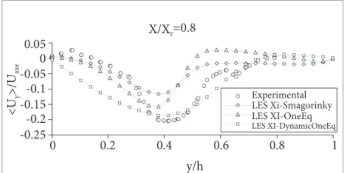
h e values of the normal velocity component at X/Xr=0.8 are presented in Fig. 19. h e one equation and the Smagorinsky models are in good agreement with the experimental results in the region behind the obstacle (y/h<0.4), while the dynamic model underpredicts the experimental results. Away from the central region, approaching the upper wall, the trend is reversed and the dynamic model shows better results than the Smagorinsky and one equation models. h ese results are not conclusive to which turbulence model is more suitable for the reactive case simulation. h is same behavior is also observed for the normal velocity component at X/Xr=1.4 (Fig. 20), with dif erent turbulent models performing better or worse at dif erent regions of the l ow domain, but all models capturing the general trends of the experimentally observed velocity distributions.
h e progress variable computed by the dynamic model is presented in Figs. 21 and 22 and compared to the experimental distribution. h e simulation captures the general behavior of the progress variable quite well. Despite the fact that the simulation overpredicts the progress variable inside the l ame zone, the l ame front at c=0.05 around y/h=0.6 matches the experimental value in X/Xr=0.35 and underpredicts for X/ Xr=1.4. Also, Sanquer (1998) states that the experimental results seem to be displaced to the let .
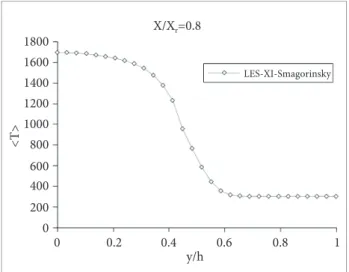
For the 3-D reactive case, a value of 1,750K was obtained for the flame average temperature with the dynamic model. The theoretical adiabatic flame temperature for a equivalence ratio of 0.65 corresponds to 1,750K for this fuel. Figures 23 and 24 show the temperature distribution in the normal direction with a profile corresponding to a premixed flame.
The vorticity distribution in the inert and reactive cases can be compared with the help of Figs. 25 and 26. These figures show the flow structure in the (x, y) cut at the center of the channel. As in Park’s discussion (Park and Ko 2011), the chemical reaction has a stabilizing effect on the vortex shedding.
-0.5 -1 1 2 1.5
0.5 0
0 0.2 0.4 0.6 0.8 1
X/Xr=0.8
y/h
LES Xi-Smagorinky LES XI-OneEq
LES XI-DynamicOneEq
Experimental
<U
x
>/U
axe
Figure 17. Mean longitudinal velocity proi le Ux at X/Xr=0.8. Reactive case.
-0.5 1 2 1.5
0.5 0
0 0.2 0.4 0.6 0.8 1
X/Xr=1.4
y/h
LES Xi-Smagorinky LES XI-OneEq
LES XI-DynamicOneEq
Experimental
<U
x
>/U
axe
Figure 18. Mean longitudinal velocity proi le Ux at X/Xr=1.4. Reactive case.
0.05 0 - 0 .0 5
-0.1
-0.2 -0.25 -0.15
0 0.2 0.4 0.6 0.8 1
X/Xr=0.8
y/h
<U
y
>/U
axe
LES Xi-Smagorinky LES XI-OneEq
LES XI-DynamicOneEq
Experimental
Figure 19. Mean normal velocity proi le Uy at X/Xr=0.8. Reactive case.
-0.1 -0.2
-0.3 0.1 0
0 0.2 0.4 0.6 0.8 1
X/Xr=1.4
y/h
LES Xi-Smagorinky LES XI-OneEq
LES XI-DynamicOneEq
Experimental
<U
y
>/U
axe
Figure 20. Mean normal velocity proi le Uy at X/Xr=1.4.
h e inert case clearly shows the Karman vortex street behind the bluf body, while in the reactive case the characteristic alternating vortex structure starts further downstream with a much weaker strength. h e vorticity near the bluf body has a stretched topology on the reactive case and the wake spreading is lower than the wake spreading of the inert case, which is in agreement with the behavior described by Park and Ko (2011).
CONCLUSIONS
Results from numerical simulations of inert and reactive l ows were compared to experimental results obtained by Sanquer
0 200 400 600 800 1000 1200 1400 1600 1800
0
X/Xr=0.8
y/h
LES-XI-Smagorinsky
<T>
0.2 0.4 0.6 0.8 1
Figure 23. Mean temperature proi le at X/Xr=0.8.
0.8 1
0.6
0.4
0.2
0 0
X/Xr=1.4
y/h
LES-XI-Smagorinsky Experimental
<C>
0.2 0.4 0.6 0.8 1
Figure 22. Proi le of the progress variable at X/Xr=1.4.
0.8 0.7
0.5
0.3
0.1 0.6
0.4
0.2
0 0
X/Xr=0.35
y/h
LES-XI-Smagorinsky Experimental
<C>
0.2 0.4 0.6 0.8 1
Figure 21. Proi le of the progress variable at X/Xr=0.35.
Figure 24. Temperature contours behind the bluff body.
Figure 25. Inert l ow spanwise vorticity.
(1998). Smagorinsky, one equation and dynamic LES models were used and the reaction was simulated using the Ξ density of wrinkling model. he experiments are in the thin, wrinkled lame regime with a Re of 6,690, a Da of 4.5 and a Ka of 1.3.
For the inert low case, the simulations using LES good results were obtained for the St, with an error of the order of 3%. he size of the recirculation bubble is close to the size observed experimentally but the margin of error is larger, around 12%. But these values are not absolute values since the experimental results also have a margin of error. he energy decay on the inertial range was correctly captured at -5/3. As far as the velocity distribution is concerned, the streamwise velocity component shows good agreement with the experimental values, but the normal velocity components are somewhat of, in part as a consequence of the over-predicted recirculation zone length.
he results for the reactive low case show similar performance with the inert case. he energy decay rate in the inertial range was correctly captured and the vortex sheading frequency was close to the experimental value. he progress variable and the correct behavior considering the stabilization
of the vortex sheading behind the obstacle for the reactive case were captured by the simulation. Again, on the reactive case, the velocity distribution was somewhat of from the experimental measurements. Regarding the velocity proile, it is still interesting to observe that the SM gives a better result than the dynamic model used in these simulations. he results may be improved by tailoring the dynamic turbulent model coeicients. In general, the results for all three models are relatively similar and the diferences between these models are small. herefore, since the dynamic model has a higher computational cost, it may be worthwhile to use the Smagorinsky or the one equation model.
ACKNOWLEDGMENTS
he authors would like to thank the Instituto de Aeronáutica e Espaço for the use of their computational facilities in the Laboratory of Liquid Propulsion and Brazilian Government CAPES for the inancial support.
REFERENCES
Akula, R.A., Sadiki, A. and Janicka, J., 2006, “Large Eddy Simulation of Bluff Body Stabilized Flame by Using Flame Surface Density Approach”. Proceedings of the European Conference on Computational Fluid Dynamics. ECCOMAS CFD.
Bai, X.S. and Fuchs, L., 1994, “Modeling of turbulent reactive lows past a bluff body: Assessment of accuracy and eficiency”. Computers & Fluids, Vol. 23, No. 3, pp. 507-521.
Borghi, R. and Destriau, M., 1998, “Combustion and Flames: chemical and physical principles”. Éditions TECHNIP.
Boger, M. and Veynante, D., 2000, “Large eddy simulations of a turbulent premixed V-shape lame”. In: Advances in Turbulence VIII, Proceedings of the Eighth European Turbulence Conference, Barcelona, pp. 449-452.
Candel, S., 1992, “Combustion instabilities coupled by pressure waves and their active control”. Symposium (International) on Combustion, Vol. 24, No 1, pp. 1277-1296.
Chaudhuri, S., Kostka, S., Tuttle, S.G., Renfro, M.W. and Cetegen, B.M., 2011, “Blow off mechanism of two dimensional bluff body stabilized turbulent premixed lames in a prototypical combustor”. Combustion and Flame, Vol. 158, No 7, pp. 1358-1371.
Cheng, R.K., 1984, “Conditional sampling of turbulence intensities and Reynolds stress in premixed turbulent lames”. Combustion Science and Technology, Vol. 41, pp.109-142.
Cheng, R.K., Shepherd, I.G. and Gokalp, I., 1989, “A comparison of the velocity and scalar spectra in premixed turbulent lames”. Combustion and Flame, Vol.78, No 2, pp. 205-221.
Cheng, R.K. and Shepherd, I.G., 1991, “The inluence of burner geometry on premixed turbulent lame propagation”. Combustion and Flame, Vol. 85, No 1-2, pp. 7-26.
Dourado, W.M.C., 2003, “Desenvolvimento de um método numérico em malhas não estruturadas híbridas para escoamentos turbulentos em baixo número de Mach: aplicação em chama propagando-se livremente e esteiras inertes e reativas”. Tese (Doutorado), Instituto Tecnológico de Aeronáutica, São José dos Campos.
Eriksson, P., 2007, “The Zimont TFC model applied to premixed bluff body stabilized combustion using four different RANS turbulence models”. Proceedings of ASME GT2007, ASME Turbo Expo 2007, Vol. 2, pp. 353-361, Montreal.
Frendi, A., Skarath, G. and Tosh, A., 2004, “Prediction of noise radiated by low over a smooth square cylinder”. Proceedings of the 10th AIAA/CEAS Aeroacoustics Conference, Manchester, UK.
Fureby, C., Tabor, G., Weller, H.G. and Gosman, A.D., 1997, “A comparative study of subgrid scale models in homogeneous isotropic turbulence”. Physics of luids, Vol. 9, No 5, pp. 1416-1429.
Ghosal, S., Lund, T., Moin, P. and Akselvoll, K., 1995, “A dynamic localization model for large-eddy simulation of turbulent lows”. Journal of Fluid Mechanics, Vol. 286, pp. 229-255.
Jayatilleke, C., 1969, “The inluence of prandtl number and surface roughness on the resistance of the laminar sublayer to momentum and heat transfer”. Prog. Heat Mass Transfer, Vol. 1, pp. 193-321.
Kerstein, A.R., 1989, “Linear-eddy modeling of turbulent transport II. Application to shear layer mixing”, Combustion and Flame, Vol. 75, No 3-4, pp. 397-413.
Kiel, B., Garwick, L.K., Gord, J.G., Miller, J. and Lynch, A., 2007, “A detailed investigation of bluff body stabilized lames”. AIAA 2007-168, Proceedings of the 45th AIAA Aerospace Sciences Meeting and Exhibit 8 - 11 January 2007, Reno, Nevada.
Lovett, J.A., Brogan, T.P., Philippona, D.S., Keil, B.V. and Thompson, T.V., 2004, “Development Needs for Advanced Afterburner Designs”, Proceedings of the 40th AIAA/ASME/SAE/ASEE Joint Propulsion Conference & Exhibit, Fort Lauderdale, Florida.
Manickam, B., Franke, J., Muppala, S.P. and Dinkelacker, F., 2012, “Large-eddy Simulation of Triangular-stabilized Lean Premixed Turbulent Flames: Quality and Error Assessment”. Flow, Turbulence and Combustion. Vol. 88, No 4, pp. 563-596.
Menon, S., McMurtry, P.A. and Kerstein, A.R., 1993, “A linear eddy mixing model for large eddy simulation of turbulent combustion”, In: Galperin, B. and Orszag, S. (Eds.), “Large Eddy Simulation of Complex Engineering and Geophysical Flows”, Cambridge University Press, Cambridge, pp. 287-314.
Park, N.S. and Ko, S.C., 2011, “Large eddy simulation of turbulent premixed combustion low around bluff body”. Journal of Mechanical Science and Technology, Vol. 25, No 9, pp. 2227-2235.
Peters, N., 2000, “Turbulent Combustion”, Cambridge University Press, Cambridge.
Pope, S.B., 2000, “Turbulent Flows”. Cambridge University Press, Cambridge.
Porumbel, I. and Menon S., 2006, “Large Eddy Simulation of Bluff Body Stabilized Premixed Flame”, AIAA 2006-152.
Sanquer, S., 1998, “Experimental Study of a Bluff Body Wake, in Presence of Combustion, in Fully Developed Turbulent Channel Flow. Turbulence Scales and Critical Analysis of Transport and Combustion
Models”, Ph.D. Thesis, Université de Poitiers, Potiers.
Saghaian, M., Stansby, P.K., Saidi M.S. and Apsley, D.D., 2003, “Simulation of turbulent lows around a circular cylinder using nonlinear eddy viscosity modelling: steady and oscillatory ambient lows”. Journal of Fluids and Structures, Vol. 17, No 8, pp. 1213-1236.
Sjunesson, A., Henriksson, R. and Lofstrom, C., 1992, “Cars measurements and visualization of reacting lows in bluff body stabilized lame”. AIAA-92-3650.
Sjunnesson, A., Olovsson, S. and Sjoblom, B., 1991, “Volvo Flygmotor internal report”, VFA9370-308.
Tabor, G. and Weller, H.G., 2004, “Large eddy simulation of premixed turbulent combustion using Xi lame surface wrinkling model”. Flow, Turbulence and Combustion, Vol. 72, pp. 1-28.
Tabor, G.R. and Baba-Ahmadi, M.H., 2010, “Inlet conditions for large eddy simulation: a review”. Computers & Fluids, Vol. 39, No 4, pp. 553-567.
Veynante, D., 2006, “Large eddy simulation of turbulent combustion”. Conference on Turbulence and Interaction, Vol. TI 2006, p. 20, Porquerolles, France.
Weller, H.G., Marooney, C.J. and Gosman, A.D., 1990, “A new spectral method for calculation of the time varying area of laminar lame in homogeneous turbulence”. Proceedings of the 23rd Symposium (International) on Combustion, The Combustion Institute, Vol. Twenty-third Symposium, pp. 629-636.
Weller, H.G., 1993, “The development of a new lame area combustion model using conditional averaging”. Thermo-Fluids Section Report TF 9307, Imperial College of Science, Technology and Medicine, London.
Weller, H.G., Tabor, G., Gosman, A. and Fureby, C., 1998, “Application of a lame-wrinkling les combustion model to a turbulent mixing layer”, Symposium (International) on Combustion, The combustion Institute, Vol. 27, No 1, pp. 899-907.
Yoshizawa, A. and Horiuti, K., 1985, “A statistically-derived subgrid-scale kinetic energy model for the large-eddy simulation of turbulence lows”. Journal of Physical Society of Japan, Vol. 54, pp. 2834-2839.