www.biogeosciences.net/10/6989/2013/ doi:10.5194/bg-10-6989-2013
© Author(s) 2013. CC Attribution 3.0 License.
Biogeosciences
Estimating global carbon uptake by lichens and bryophytes with a
process-based model
P. Porada1, B. Weber2, W. Elbert2, U. Pöschl2, and A. Kleidon1
1Max Planck Institute for Biogeochemistry, P.O. Box 10 01 64, 07701 Jena, Germany 2Max Planck Institute for Chemistry, P.O. Box 3060, 55020 Mainz, Germany
Correspondence to:P. Porada ([email protected])
Received: 14 January 2013 – Published in Biogeosciences Discuss.: 28 February 2013 Revised: 24 July 2013 – Accepted: 23 August 2013 – Published: 5 November 2013
Abstract.Lichens and bryophytes are abundant globally and
they may even form the dominant autotrophs in (sub)polar ecosystems, in deserts and at high altitudes. Moreover, they can be found in large amounts as epiphytes in old-growth forests. Here, we present the first process-based model which estimates the net carbon uptake by these organisms at the global scale, thus assessing their significance for biogeo-chemical cycles. The model uses gridded climate data and key properties of the habitat (e.g. disturbance intervals) to predict processes which control net carbon uptake, namely photosynthesis, respiration, water uptake and evaporation. It relies on equations used in many dynamical vegetation mod-els, which are combined with concepts specific to lichens and bryophytes, such as poikilohydry or the effect of wa-ter content on CO2diffusivity. To incorporate the great func-tional variation of lichens and bryophytes at the global scale, the model parameters are characterised by broad ranges of possible values instead of a single, globally uniform value. The predicted terrestrial net uptake of 0.34 to 3.3 Gt yr−1of carbon and global patterns of productivity are in accordance with empirically-derived estimates. Considering that the as-similated carbon can be invested in processes such as weath-ering or nitrogen fixation, lichens and bryophytes may play a significant role in biogeochemical cycles.
1 Introduction
Lichens and bryophytes are different from vascular plants: Lichens are not real plants, but a symbiosis of a fungus and at least one green alga or cyanobacterium, whereas bryophytes, such as mosses or liverworts, are plants which have no
spe-cialised tissue such as roots or stems. Both groups are poik-ilohydric, which means that they cannot actively control their water content because they do not have an effective epider-mal tissue, a cuticle or stomata. Mainly due to their ability to tolerate desiccation, combined with large functional vari-ation, they are extremely adaptive organisms that can cope with a great range of climatic conditions (Nash III, 1996). They grow as epiphytes on the bark or even on the leaves of trees, they cover rock outcrops and they form carpets on the forest floor at high latitudes. As a part of biological soil crusts, they also populate the surface of desert soils (Belnap and Lange, 2003).
In spite of their global abundance, however, the effect of lichens and bryophytes on global biogeochemical cycles has been examined only by a few studies. The work of Elbert et al. (2012), for instance, suggests a significant contribution of cryptogamic covers, which largely consist of lichens and bryophytes, to global cycles of carbon and nitrogen. They use a large amount of data from field experiments or lab measure-ments to estimate characteristic mean values of net carbon uptake and nitrogen fixation for each of the world’s biomes. By multiplying these mean values with the area of the respec-tive biome, they arrive at global numbers for uptake of car-bon and nitrogen. While their estimate for global net carcar-bon uptake amounts to 7 % of terrestrial net primary productivity (NPP), the derived value of nitrogen fixation corresponds to around 50 % of the total terrestrial biological nitrogen fixa-tion (BNF), representing a large impact on the global nitro-gen cycle.
of today’s lichens and bryophytes have likely contributed to the enhancement of surface weathering rates (Lenton et al., 2012). The organisms accelerate chemical weathering re-actions of the substrate by releasing organic acids, com-plexing agents, hydroxide ions or respiratory CO2 (Jack-son and Keller, 1970; Berthelin, 1988; Chen et al., 2000; Büdel et al., 2004; Weber et al., 2011). On long timescales, weathering rates of silicates control atmospheric CO2 con-centration and thus have a large influence on global cli-mate. The work of Schwartzmann and Volk (1989) shows, for example, that without biotic enhancement of weather-ing in the course of evolution, atmospheric CO2would have remained at a high level. The surface temperature associ-ated with this CO2level would probably have been too high for complex life to evolve. Lenton et al. (2012) focus on the effect of the predecessors of modern bryophytes on at-mospheric CO2 concentration during the Ordovician. Ac-cording to their experiments, these early non-vascular plants could have caused a considerable drawdown in atmospheric CO2levels via the silicate weathering feedback and, conse-quently, a decrease in global surface temperature. Further-more, the release of phosphorus from the weathered rocks into the oceans could have led to a rise in marine produc-tivity and therefore to further cooling. According to Lenton et al. (2012), this could explain two temporary glaciations at the end of the Ordovician period.
Here, we present the first process-based modelling ap-proach to estimate net carbon uptake of lichens and bryophytes at the global scale. In this way, we are able to assess the role of these organisms regarding global biogeo-chemical cycles.
Most previous modelling studies that include lichens and bryophytes focus on net primary productivity (NPP) of moss in boreal and arctic regions, especially in peatlands (see, e.g. Wania et al., 2009; Frolking et al., 2002; Yurova et al., 2007). Others focus on ecosystem responses to climate change (Bond-Lamberty and Gower, 2007; Euskirchen et al., 2009; Zhuang et al., 2006; Turetsky et al., 2012), simulating peat accumulation (Frolking et al., 2010) or peatland microtopog-raphy (Nungesser, 2003). Our model aims at a more general representation of lichens and bryophytes that makes it pos-sible to estimate the productivity of these organisms under a broad range of environmental conditions around the globe.
The model is called “LiBSi” (Lichen and Bryophyte Sim-ulator). It is similar to many global vegetation models (see Fig. 1). These models describe plants in a simplified way in-stead of simulating them with all their detailed structures. Vegetation is usually represented by a reservoir of biomass, which changes as a function of exchange flows of carbon. These exchange flows depend on processes such as pho-tosynthesis and respiration, which are represented by a set of equations. The equations use environmental factors such as radiation or water supply as input values, which are ei-ther prescribed or derived from climate forcing data. In spite of their simplicity, global vegetation models are capable of
predicting NPP to a reasonable accuracy (Randerson et al., 2009).
Similar to these models, our model describes lichens and bryophytes as reservoirs of biomass located either on the soil or in the canopy and it is based on equations to repre-sent photosynthesis and other physiological processes. These concepts are combined with properties and processes specific to lichens and bryophytes, such as the decrease of diffusiv-ity for CO2with increasing water content or the proportional relationship between metabolic activity and water saturation. The model differs from most other vegetation models with respect to the parameters contained in the model equations. Most models use parameter values that describe an “average” organism, such as a typical rain forest tree, for example. Our model uses ranges of possible parameter values which are de-rived from the literature. This approach is similar to the one used in the JeDi-DGVM (Jena Diversity-Dynamic Global Vegetation Model), which predicts global biogeochemical flows as well as biodiversity patterns (Pavlick et al., 2012). In this way, the model accounts for the large functional vari-ation of lichens or bryophytes at the global scale concerning properties such as photosynthetic capacity or specific area.
The paper is structured in the following way: Sect. 2 con-tains a description of the model, including an overview of the reservoirs and exchange flows as well as the environmen-tal factors that control these flows. In addition, the method for simulating functional variation of lichens and bryophytes by parameter ranges is explained. Estimates of net carbon uptake are presented in Sect. 3 together with an evaluation of the model performance. The model is evaluated by com-paring simulated productivity of lichens and bryophytes with observational data. Furthermore, the uncertainty regarding the values of model parameters is assessed through a sen-sitivity analysis. In Sect. 4 the plausibility of the simulated patterns of productivity is discussed. Also the limitations of the approach presented here are analysed considering the out-comes of model evaluation and sensitivity analysis. Several potential improvements of the model and its applicability to further research are discussed.
Note that we use the term “net carbon uptake” throughout the manuscript instead of “net primary productivity” (NPP). While NPP is a standard term for vascular vegetation which is frequently used in the modelling community, “net carbon uptake” is more general and descriptive. In the context of this manuscript, it corresponds to NPP.
Input Model equations Output
Climate forcing data on a global grid
Maps of environmental factors (e.g. disturbance)
Basic vegetation modelling (e.g. photosynthesis)
Lichen / Bryophyte specific traits (e.g. poikilohydry)
Exchange flows Global maps of:
Biomass reservoir
Fig. 1.Overview of the functioning of the model. Input data are translated via model equations into exchange flows of carbon, which are used to calculate changes in the biomass reservoir.
2 Model description
Lichens and bryophytes are described in the model by a reservoir approach, which means that they are repre-sented by pools of chemical substances. These are biomass, sugar reserves, water and internal CO2 concentration. Re-garding lichens, the biomass of the fungal and the al-gal/cyanobacterial partner are simulated in an aggregated form as one pool of biomass with average properties.
Changes in the size of the pools are due to input and output flows of carbon or water. Carbon is assimilated by photosyn-thesis from the atmosphere and temporarily stored as sugars. The sugars are then respired for maintenance or transformed into biomass. Water is taken up and evaporates via the thallus surface. The water content of the thallus influences several physiological processes, such as CO2diffusion.
The processes which determine the carbon and water flows are driven by climate. In addition to the climate forcing, properties of the living environment also affect lichens and bryophytes in the model. These properties depend on the lo-cation of growth, which is either the canopy or the ground, as well as the surrounding vegetation, which is described by a biome classification.
2.1 Model processes
In the following, we describe the physiological processes im-plemented in the model. First, we name the effects of the liv-ing environment on lichens and bryophytes. Then, we explain how water content and climatic factors relate to physiological properties of the organism. Finally, we describe the exchange flows between the organism and its environment.
For simplicity, we will not present any equations. All equa-tions used in the model can be found in Appendix B and are explained there. The parameters associated with the equa-tions are listed in Tables B7 to B13 in the appendix.
2.1.1 Living environment
In the model, lichens and bryophytes can be located either in the canopy or on the ground. The location of growth is important for the radiation and precipitation regime the or-ganism is exposed to (see Fig. 2). Lichens and bryophytes living in the upper part of the canopy, for example, may re-ceive more shortwave radiation than those living beneath the canopy. Additionally, the location of growth determines the available area for growth. The available area in the canopy is assumed to be the sum of leaf area index (LAI) and stem area index (SAI). The available area on the ground depends on (a) the amount of soil not occupied by other vegetation and (b) LAI, since the litter layer resulting from leaf fall impedes the growth of lichens and bryophytes (see Fig. 2). Once a lichen or bryophyte covers the available area completely, it cannot grow anymore. Since the biomass of an organism is related to its surface area, biomass is also limited by the available area.
Another factor that shapes the living environment of lichens and bryophytes is the biome where the organisms are located. In the model, the biome controls the frequencies of disturbance events, such as fire or treefall, for instance. Furthermore, both location of growth and biome determine the aerodynamic roughness of the surface where lichens or bryophytes grow. A forest, for example, has a higher rough-ness than a flat desert. Together with wind speed, surface roughness has a large impact on the aerodynamic resistance to heat transfer between the surface and the atmosphere (Allen et al., 1998). Lichens and bryophytes in the canopy of an open forest, for instance, exchange heat faster than those on the flat surface of a desert.
2.1.2 Water relations
Available area
on canopy
Available area on ground
Partitioning =
f
(LAI)
Precipitation
Radiation
occupied
Leaf fall
Fig. 2.Effect of the leaf area index (LAI) on area for growth and climate forcing. Available area on ground is a linearly decreasing function of LAI. The same function is used to partition precipitation between canopy and soil. The vertical distribution of light is calculated according to Beer’s law as a function of LAI.
where the latter is proportional to biomass. The water satura-tion controls three important physiological properties:
1. The diffusivity of the thallus for CO2, which is in-versely related to water saturation since water leads to a swelling of cells and thus to a narrowing of the diffusion pathways (Cowan et al., 1992);
2. The water potential, which increases from−∞at zero
water saturation to a maximum value of 0 at a certain threshold saturation. If the water saturation is above this threshold, all cells in the thallus are fully turgid and extracellular water may exist inside the thallus or on its surface; and
3. The metabolic activity of a lichen or bryophyte, which determines both the relative strength of photosynthe-sis as well as that of respiration as a function of wa-ter saturation (Lange, 1980, 2002; Lidén et al., 2010; Williams and Flanagan, 1998). The metabolic activity is assumed to increase linearly from 0 at zero water saturation to 1 at the threshold saturation. It remains 1 if the water saturation exceeds the threshold saturation. This relation accounts for the fact that water is needed in the cells of the organism to activate enzymes and to enable chemical reactions.
Note that the water relations implemented in the model al-low for representation of the species-specific dependency of photosynthesis on water content. At low water content, pho-tosynthesis is limited by metabolic activity, while at higher water content it is limited by the diffusivity of the thallus for CO2. Depending on the relative strength of these limitations, different shapes of the relation between photosynthesis and water content can be simulated.
2.1.3 Climate relations
The climate forcing consists of air temperature, wind speed, relative humidity, precipitation and downwelling short- and longwave radiation. These climatic factors influence ex-change flows of carbon and water between lichens and bryophytes and their environment. Furthermore, the cli-matic factors directly control two physiological properties of lichens and bryophytes, namely potential evaporation and surface temperature.
Both potential evaporation and surface temperature are calculated according to Monteith (1981) as a function of four factors:
1. Net radiation, which is the sum of downwelling short-and longwave radiation, upwelling longwave radiation and the ground heat flux;
2. Saturation vapour pressure, which is calculated as a function of air temperature (Allen et al., 1998). It is also influenced by the water potential of a lichen or bryophyte (Nikolov et al., 1995);
3. Aerodynamic resistance to heat transfer; and 4. Relative humidity.
Additionally to the climate forcing, physiological pro-cesses of lichens and bryophytes are affected by the presence of snow. If the snow layer exceeds a certain thickness, it is as-sumed that the metabolism of the organisms is reduced due to lack of light and low temperature.
2.1.4 Exchange flows
in Fig. 3 together with relations to climate forcing and reser-voirs inside the thallus.
The inflow of CO2 into the pore space of the lichen or bryophyte depends on the gradient between the partial pres-sure of CO2in the atmosphere and in the pore space as well as the diffusivity of the thallus for CO2.
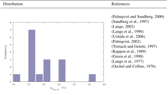
The uptake of CO2 from the pore space (gross primary productivity, GPP) is computed as a minimum of a light-limited rate, which depends on intercepted shortwave radi-ation, and a CO2-limited rate, which is a function of pore space CO2(Farquhar and von Caemmerer, 1982). Both rates also depend on the surface temperature of the organism (Medlyn et al., 2002) and its metabolic activity status. Pho-tosynthesis is assumed to peak around an optimum surface temperature (June et al., 2004).
Respiration is modelled by a Q10relationship as a function of biomass and temperature (Kruse et al., 2011). Same as GPP, it too depends on metabolic activity. The respired CO2 is released into the pore space.
Hence, the CO2 balance of the lichen or bryophyte pore space is controlled by inflow, GPP and respiration. GPP is added to the sugar reservoir, while respiration is subtracted. Then, a certain fraction of the sugar reservoir is transformed into biomass with a certain efficiency. This constitutes the net primary productivity (NPP). The balance of the biomass reservoir is then determined by NPP and biomass loss, which includes regular processes such as tissue turnover or leach-ing of carbohydrates (Melick and Seppelt, 1992). Addition-ally, disturbance events which occur at characteristic time in-tervals lead to a reduction of biomass.
Evaporation from the lichen or bryophyte thallus is com-puted as a minimum of water content and potential evapo-ration. Since lichens and bryophytes cannot actively control water loss, evaporation is not affected by the activity status of the organism. Water uptake takes place via the thallus sur-face. Where water input exceeds maximum storage capacity, surplus water is redirected to runoff. The water balance of the lichen or bryophyte is thus determined by evaporation and water uptake.
2.2 Model parameters
The equations that describe physiological processes in the model are parameterised and the parameters can be sub-divided into two categories: (1) properties of lichens and bryophytes, and (2) characteristics of the environment of the organisms. Since lichens and bryophytes have a large func-tional variation, the parameters that represent their proper-ties, such as specific area or photosynthetic capacity, are characterised by large ranges of possible values. To incor-porate the functional variation of lichens and bryophytes into the model, many physiological strategies are gener-ated by randomly sampling the ranges of possible parame-ter values. We call these parameparame-terisations “strategies” and not “species” because they do not correspond exactly to
any species that can be found in nature. Nevertheless, these strategies are assumed to represent the physiological proper-ties of real lichen and bryophyte species in a realistic way. Hence, the functional variation of the organisms can be sim-ulated without knowing the exact details of each species.
The model is then run with all strategies, but not every strategy is able to maintain a positive biomass in each grid cell, which is necessary to survive. The results are computed by averaging only over the surviving strategies of each grid cell. Thus, climate is used as a filter to narrow the ranges of possible parameter values in each grid cell and therefore to make the results more accurate (see Fig. 4).
The studies of Bloom et al. (1985); Hall et al. (1992) anal-yse from a theoretical perspective the relations between the “strategy” of an organism and the success of this organism regarding natural selection in a certain environment. Follows and Dutkiewicz (2011) apply this approach to marine ecosys-tems, while Kleidon and Mooney (2000) use it to predict bio-diversity patterns of terrestrial vegetation. The applicability of this method to modelling biogeochemical fluxes of terres-trial vegetation has been successfully demonstrated by the JeDi-DGVM (Pavlick et al., 2012).
The 15 model parameters which are included in the ran-dom sampling method are listed in Table B9 in the appendix. They represent structural properties of the thallus of a lichen or bryophyte, such as specific area or water storage capacity. They also describe implications of the thallus structure, such as the relation between water content and water potential. Furthermore, characteristics of the metabolism are consid-ered, such as optimum temperature. Parameters which have categorical values are also used: a lichen or bryophyte can ei-ther live in the canopy or at the soil surface (see Sect. 2.1.1). Another categorical parameter determines if the organism has a carbon concentration mechanism (CCM) or not. For the model, it is assumed that the CCM in lichens works sim-ilarly to those in free-living cyanobacteria. Based on this as-sumption, the CCM implemented in our model represents an advantage for the organisms in cases of low internal CO2 concentrations in a water saturated thallus. Although regu-lation of the CCM has been observed (Miura et al., 2002), the model contains a fixed representation of the CCM for simplicity.
Some of the 15 parameters mentioned above are related to further lichen or bryophyte parameters. The respiration rate at a certain temperature, for instance, is assumed to be re-lated to Rubisco content and turnover rate. Hence, the pa-rametersRubisco contentandturnover rateare not sampled
from ranges of possible values, but determined by the value of the parameter respiration rate. The reason for this
Input data
Flows Reservoirs Processes Effects
CO2
[ CO2 ]
H2O
Biomass
Sugars NPP
Biomass loss
GPP Runoff
Heat Precipitation Light
Photosynthesis Respiration
TAir & Humidity & Wind
Evaporation
Water uptake
Disturbance Living environment
TSurface
Fig. 3.Schematic of the carbon and water relations of a lichen or bryophyte simulated by the model. Dotted arrows illustrate effects of climate forcing, living environment and state variables on physiological processes of a lichen or bryophyte. These processes are associated with exchange flows (solid arrows) of carbon (black), water (blue) and energy (red).
respiration, while only the algal/cyanobacterial biomass con-tains Rubisco. In the model, however, lichen respiration is assumed to be controlled by the Rubisco content averaged over the total biomass.
The relationships between parameters are called tradeoffs and they are assumed to have constant values. This means that although the value of one parameter (e.g. Rubisco con-tent) may vary across species, the tradeoff-function which relates this parameter to another one (e.g. respiration) should be more or less the same for many different species.
Six tradeoffs are implemented in the model. The first tradeoff describes the relation between Rubisco content, res-piration rate and turnover rate explained above. The second tradeoff relates the diffusivity for CO2to the metabolic ac-tivity of the lichen or bryophyte via its water content. This means that a high diffusivity is associated with a low water content, which results in a low activity. The third tradeoff de-scribes the positive correlation between the maximum elec-tron transport rate of the photosystems (Jmax) and the maxi-mum carboxylation rate (VC, max). Since both rates represent costs for the organism and photosynthesis is the minimum of the two, it would be inefficient if they were independent from each other. The fourth tradeoff is associated with the carbon concentration mechanism (CCM). In case a lichen or bryophyte possesses a CCM, a part of the energy acquired by the photosystems is not used to fix CO2, but rather to increase
the CO2concentration in the photobionts. If the organism is limited by low CO2 but enough light is available, a CCM can lead to higher productivity. The fifth and sixth tradeoffs concern the Michaelis–Menten constants of the carboxyla-tion and oxygenacarboxyla-tion reaccarboxyla-tions of Rubisco. They relate these constants to the molar carboxylation and oxygenation rates of Rubisco. One tradeoff is usually associated with more than one parameter. The model parameters that describe tradeoffs are listed in Table B10.
The model contains several additional lichen or bryophyte parameters which are not directly associated with tradeoffs, but which represent physiological or physical constraints. Therefore, they are assumed to have constant values. They can be found in Table B11.
Rubisco content
Specific area
Strategy no. 1
Strategy no. 2 Range of possible values
...
Hot desert
Moist forest a)
b)
Fig. 4.Generation of physiological strategies and their survival. (a)Many random parameter combinations (strategies) are sampled from ranges of possible values. The strategies are then run in each grid cell of the model.(b)Example: In a hot desert, strategy 1 sur-vives because a small specific area reduces water loss by evapora-tion and a high Rubisco content is adequate to high intensities of light. Strategy 2, however, dies out since too much water evapo-rates due to a large specific area. In a moist forest, strategy 1 dies out because a high Rubisco content is associated with high respi-ration costs which cannot be covered by low light conditions under a canopy. Strategy 2 can survive since it does not have high respi-ration costs. Note that these examples are not generally applicable. High specific area, for instance, could also be useful in a desert to collect dew.
age, for example, which are not considered in the model. Hence, snow density is set to a constant global average value. For a list of parameters related to environmental conditions, see Table B8.
2.3 Simulation setup
The model runs on a global rectangular grid with a resolution of 2.8125 degrees (T42); hence, all input data are remapped to this resolution. The land mask and the climate forcing are taken from the WATCH data set (Weedon et al., 2011). This data set comprises shortwave radiation, downwelling longwave radiation, rainfall, snowfall, air temperature at 2 m height, wind speed at 10 m height, surface pressure and spe-cific humidity. The latter two variables are used to compute relative humidity. The temporal resolution of the data is 3 h and the years 1958–2001 are used. Since the model runs on an hourly time step, the data are interpolated. In addition to the climate forcing, the model uses maps of LAI and SAI in a monthly resolution and a temporally constant map of bare soil area, all of which are taken from the Community Land Model (Bonan et al., 2002). They are used to provide esti-mates for the available area for growth and the light environ-ment. A biome map taken from Olson et al. (2001) is used to represent disturbance by assigning characteristic disturbance intervals to each biome (see Table B3). Furthermore, surface roughness is determined as a function of the biome.
The model provides output for each surviving strategy in a grid cell independently. Hence, to obtain an average output value for a certain grid cell, the different strategies have to be weighted. Since ecological interactions between species are not considered in the model, it is not possible to determine the relative abundance and thus the weight of each strategy. Therefore, the uncertainty due to the unknown weights of the strategies has to be included into the results. As a lower bound for net carbon uptake in a certain grid cell, we assume that all strategies are equally abundant and the estimate thus corresponds to equal weights for all surviving strategies. This weighting method is called “average”. Since strategies that do not grow much are probably not as abundant as strongly growing strategies, the true net carbon uptake is probably un-derestimated by this method. As an upper bound we assume a weight of one for the strategy with the highest growth and zero for all other strategies. This weighting method is called “maximum” and it is probably an overestimate of the true value since competition between species would have to be very strong to reduce diversity to such an extent. The upper and lower bounds derived from the two weighting methods are then used for the evaluation of the model.
The studies selected for the model–data comparison are limited to those which report estimates of average, long-term net carbon uptake based on surface coverage of lichens or bryophytes. Studies which estimate only maximum rates of carbon uptake or carbon uptake per area lichen/bryophyte or per gram biomass cannot be used. To include such studies, we would have to make assumptions about the active time of lichens and bryophytes throughout the year, about their ground coverage, etc. Hence, we would not compare our modelled estimates to data but to another, empirical model. Our criteria lead to the exclusion of many studies which mea-sure productivity of lichens and bryophytes. Consequently, only 4 out of 14 biomes are represented in the field studies: tundra, boreal forest, desert and tropical rainforest.
For a list of studies used in the model–data comparison, see Table 1. The list does not comprise all existing studies which provide observational data on net carbon uptake of lichens and bryophytes. In our opinion, however, it is suf-ficient to illustrate the order of magnitude of net carbon up-take.
The model is run for 2000 yr with an initial number of 3000 strategies. The simulation length of 2000 yr is sufficient to reach a dynamic steady state regarding the carbon balance of every strategy, which also implies that the number of sur-viving strategies has reached a constant value. Furthermore, the initial strategy number of 3000 is high enough to achieve a representative sampling of the ranges of possible parame-ter values. This means running the model with 3000 different strategies leads to a very similar result. The model output is averaged over the last 100 years of the simulation, since this period corresponds to the longest disturbance interval in the model. The simulation described above takes 7 days on 48 processors of a parallel computer. The source code (written in Fortran 95) is available on request.
3 Results
The model presented here is designed to predict global net carbon uptake by lichens and bryophytes. The predicted val-ues are shown in the form of maps as well as global aver-age numbers. Additionally, further properties of lichens and bryophytes estimated by the model are presented to illustrate the large range of possible predictions. To assess the qual-ity of the predictions, the model estimates are compared to observational data.
To estimate the effect of uncertain model parameter val-ues on the predictions of the model, a sensitivity analysis is performed.
3.1 Modelled net carbon uptake
The global estimate of net carbon uptake by lichens and bryophytes amounts to 0.34 (Gt C) yr−1 for the average-weighting method and 3.3 (Gt C) yr−1 for the
maximum-Table 1.Overview of the studies used to evaluate the model. The value in brackets in the column “Net carbon uptake” corresponds to the number of observations contained in the respective study. A ⋆-symbol denotes studies which provide one or more ranges instead of single values. In these cases, we calculated the mean value of the upper and lower bound of each range and show the range of these calculated mean values in the table. If net carbon uptake was reported in units of gram biomass, we used a factor of 0.4 (relative weight of carbon in CH2O) as a conversion factor for carbon.
Study Biome Net carbon uptake [(g C) m−2yr−1] (Billings, 1987) Tundra 10 (Lange et al., 1998) Tundra 4.7–20.4 (4) (Oechel and Collins, 1976) Tundra 38.5–171 (2) (Schuur et al., 2007) Tundra 12–60 (3) (Shaver and Chapin III, 1991) Tundra 2–68 (4) (Uchida et al., 2006) Tundra 1.9 (Uchida et al., 2002) Tundra 6.5 (Billings, 1987) Boreal forest 9.7–78 (2) (Bisbee et al., 2001) Boreal forest 25 (Camill et al., 2001) Boreal forest 9.2–75.9 (8) (Gower et al., 1997) Boreal forest 12 (Grigal, 1985) Boreal forest 128–152 (2) (Harden et al., 1997) Boreal forest 60–280 (3)⋆ (Bond-Lamberty et al., 2004) Boreal forest 0–297.1 (14) (Mack et al., 2008) Boreal forest 0.4–16.2 (7) (Oechel and Van Cleve, 1986) Boreal forest 40–44 (2) (Reader and Stewart, 1972) Boreal forest 14.4 (Ruess et al., 2003) Boreal forest 29.2–31.2 (2) (Swanson and Flanagan, 2001) Boreal forest 104 (Szumigalski and Bayley, 1996) Boreal forest 15.2–81.2 (10) (Thormann, 1995) Boreal forest 23.2–73.2 (3) (Vogel et al., 2008) Boreal forest 12–32 (9) (Wieder and Lang, 1983) Boreal forest 216–316 (3) (Brostoff et al., 2005) Desert 11.7 (Garcia-Pichel and Belnap, 1996) Desert 0.54 (Jeffries et al., 1993) Desert 0.07–1.5 (3)⋆ (Klopatek, 1992) Desert 5.3–29 (4)⋆ (Clark et al., 1998) Tropical forest 37–64 (2)
weighting method (for a description of these weighting meth-ods see Sect. 2.3). The global biomass is 4.0 (Gt C) (average) and 46 (Gt C) (maximum), respectively.
We show maps of the global net carbon uptake by lichens and bryophytes, biomass, surface coverage, number of sur-viving strategies and two characteristic parameters, the opti-mum temperature of gross photosynthesis and the fraction of organisms with a carbon concentration mechanism (CCM). These maps are created from time averages over the last 100 yr of the simulation described in Sect. 2.3. The maps are based on the average-weighting method. The maximum-weighting shows very similar patterns and the corresponding maps are shown in Fig. A1a–d.
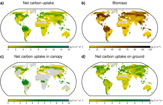
the lowest productivity, the highest values are reached in the boreal zone and in the moist tropics. In the tropical rainforest the high productivity is mainly due to the high carbon uptake by epiphytic lichens and bryophytes (see Fig. 5c). In the bo-real zone, lichens and bryophytes in the canopy as well as on the ground contribute significantly to carbon uptake (see Fig. 5d). Biomass (Fig. 5b) exhibits a global pattern simi-lar to carbon uptake. At high latitudes, however, the ratio of biomass to carbon uptake seems to be slightly higher than in the tropics.
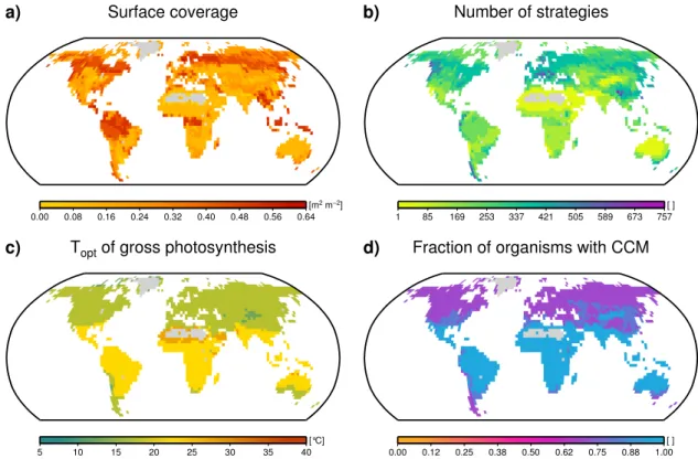
Figure 6a shows the global absolute cover of lichens and bryophytes in m2projected surface area of the organisms per m2 ground. Since the available area can be higher than one in the canopy, high values of absolute cover do not neces-sarily mean high fractional cover. On the contrary, the frac-tional cover is highest in regions with low absolute cover, especially grasslands and agricultural areas, since the avail-able area in these regions is very small. A map of fractional cover is shown in Fig. A2. Figure 6b shows the number of surviving strategies at the end of the simulation. The global pattern is slightly different from the pattern of carbon up-take. Although forested regions show the highest number of strategies, the high latitudes are richer in strategies than the tropics.
Figures 6c and d show the global patterns of two char-acteristic lichen and bryophyte parameters. As described in Sect. 2.2, these parameters are sampled randomly from ranges of possible values to create many artificial strategies. Thus, at the start of a simulation, possible values from the range of a certain parameter are present in equal measure in each grid cell. During the simulation, however, parame-ter values from certain parts of the range might turn out to be disadvantageous in a certain climate and the correspond-ing strategies might die out. This leads to a narrowcorrespond-ing of the range and consequently to global patterns of characteristic parameters. These patterns reflect the influence of climate on properties of surviving strategies. Figure 6c shows the op-timum temperature of gross photosynthesis of lichens and bryophytes living on the ground. The optimum temperature shows a latitudinal pattern, with high values in the tropics and low values towards the poles or at high altitudes. Figure 6d shows the fraction of organisms on the ground that have a carbon concentration mechanism (CCM). This parameter is also characterised by a latitudinal pattern. The fraction of or-ganisms with a CCM is almost one in the tropics, while it is approximately 0.5 in polar regions. Lichens and bryophytes living in the canopy exhibit global patterns of optimum tem-perature and CCM fraction similar to those living on the ground. The corresponding maps are shown in Fig. A2.
3.2 Evaluation
Figure 7 shows a comparison between model estimates and observational data with regard to net carbon uptake for four biomes. As discussed in Sect. 2.3, the observational data are
point-scale measurements which show high variation. There-fore, the median of the observed values from a biome is used as a characteristic value of net carbon uptake. This median value is compared to the upper and lower bound of simulated net carbon uptake averaged over the biome (see Sect. 2.3 for a description of how the bounds are derived). Also shown is the variation of carbon uptake between the most- and the least-productive grid cell in a biome for both bounds of the model estimates. Figure 7 illustrates that the model estimates are characterised by high variation. The range between the upper and lower bound of net carbon uptake is around one or-der of magnitude. The range of productivity of the grid cells in a biome is up to four orders of magnitude.
Considering the upper and lower bounds of simulated net carbon uptake in each biome, the model estimates agree rela-tively well with the characteristic values of net carbon uptake derived from observational data. For the boreal zone and the tropical rainforest, the characteristic values are closer to the upper bound of net carbon uptake. In the boreal zone, the data-based value matches the simulated upper bound; in the tropical rainforest it exceeds the upper bound. Possible rea-sons for these patterns are discussed in Sect. 4.
3.3 Sensitivity analysis
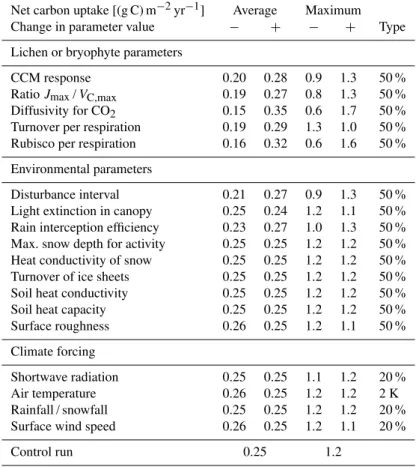
As described in Sect. 2.2, model parameters that describe tradeoffs, physiological constraints or environmental prop-erties are assumed to have constant values. Some of these parameter values have already been estimated in other stud-ies and thus they can be taken directly from the literature. Others, however, have yet to be determined. A reliable es-timate of these unknown parameter values would require a considerable amount of experimental data, which is beyond the scope of this study. Therefore, the parameter values were derived by educated guess using the available information from the literature (see Appendix B). To assess the impact of these parameter values on the model result we perform a sensitivity analysis (see Table 2). Note that some of the pa-rameters tested in the sensitivity analysis are aggregated into a single process. For a detailed overview of the parameters see Tables B8 and B10.
a) b)
c) d)
Net carbon uptake
0 2 4 6 8 10 12 14 16
[(g C) m−2yr−1]
Biomass
0 15 30 45 60 75 90 105 120
[(g C) m−2]
Net carbon uptake in canopy
0 1 2 3 4 5 6 7 8 9 10
[(g C) m−2yr−1]
Net carbon uptake on ground
0 1 2 3 4 5 6 7 8
[(g C) m−2yr−1]
Fig. 5.Global maps of model estimates.(a)Net carbon uptake by lichens and bryophytes.(b)Biomass of lichens and bryophytes.(c)Net carbon uptake by lichens and bryophytes living in the canopy.(d)Net carbon uptake by lichens and bryophytes living on the ground. The estimates are based on time averages of the last 100 yr of a 2000-yr run with 3000 initial strategies. They correspond to the average-weighting method (see Sect. 2.3). Areas where no strategy has been able to survive are shaded in grey.
the parameters. This is done to avoid generating unrealistic climatic regimes.
The turnover parameter affects maximum and average net carbon uptake in opposite ways. Moreover, the effects of the parametersJmax/VC,max, light extinction and surface rough-ness on carbon uptake are not straightforward to explain. These points are discussed in Sect. 4. For reasons of compu-tation time we used a different simulation setup (400 yr, 300 strategies) for the sensitivity analysis. Therefore, the net car-bon uptake values for the control run (Table 2) differ from the ones presented above. The pattern of productivity, however, is very similar to those of the longer run with more strate-gies (see Fig. A2). We thus assume that the sensitivity of the model does not change significantly with increased simula-tion time and number of initial strategies.
4 Discussion
In this study we estimate global net carbon uptake by lichens and bryophytes using a process-based model. In the follow-ing, we discuss the plausibility of the model estimates with respect to the patterns and the absolute values. Furthermore, we give an overview of the limits of our approach with a fo-cus on the different sources of uncertainty in the model and possible improvements.
4.1 Global patterns of net carbon uptake
a) b)
c) d)
Surface coverage
0.00 0.08 0.16 0.24 0.32 0.40 0.48 0.56 0.64 [m2m−2]
Number of strategies
1 85 169 253 337 421 505 589 673 757 [ ]
Toptof gross photosynthesis
5 10 15 20 25 30 35 40
[°C]
Fraction of organisms with CCM
0.00 0.12 0.25 0.38 0.50 0.62 0.75 0.88 1.00 [ ]
Fig. 6.Global maps of model estimates.(a)Area covered by lichens and bryophytes per m2ground.(b)Number of surviving strategies at the end of a model run.(c)Optimum temperature of gross photosynthesis of lichens and bryophytes on the ground.(d)Fraction of lichens and bryophytes on the ground with a carbon concentration mechanism (CCM). The estimates are based on time averages of the last 100 yr of a 2000 yr run with 3000 initial strategies. They correspond to the average-weighting method (see Sect. 2.3). Areas where no strategy has been able to survive are shaded in grey.
these ecosystems. Hence, at a large spatial scale, the climate of the high latitudes seems to be more favourable for a large range of lichen and bryophyte growth strategies than the trop-ical climate, which is also illustrated by the higher number of strategies of the boreal forest zone compared to the tropical one. Nevertheless, the potential for productivity seems to be highest in the moist tropics, although survival in this region is more difficult.
The surface coverage shows a plausible range of values. In deserts, it is in the order of 10 % or lower and in (sub)polar regions, it is around 30 %, which seems realistic. In forested regions, it ranges from 40 to 65 %, which is plausible since the available area is larger than 1 m2 per m2 ground for lichens and bryophytes living in the canopy.
The latitudinal pattern of the optimum temperature of gross photosynthesis is realistic since the mean climate in the tropics is warmer than in polar regions or at high al-titudes. The fact that the edges of the parameter range are not represented on the map can be explained as follows: ex-treme climatic conditions, which could be associated with extreme values of the optimum temperature of gross photo-synthesis, often do not persist for long time periods. Lichens and bryophytes are usually inactive during these periods and are therefore not affected by them. Extreme temperatures that
Table 2.Influence of uncertain model parameters on simulated net carbon uptake. “Average” and “maximum” correspond to two different weighting methods for the results (see Sect. 2.3). The “+” signs denote an increase in the value of a parameter and “−” signs denote a
decrease. The rightmost column shows the type of increase or decrease.
Net carbon uptake [(g C) m−2yr−1] Average Maximum
Change in parameter value − + − + Type
Lichen or bryophyte parameters
CCM response 0.20 0.28 0.9 1.3 50 %
RatioJmax/VC,max 0.19 0.27 0.8 1.3 50 % Diffusivity for CO2 0.15 0.35 0.6 1.7 50 % Turnover per respiration 0.19 0.29 1.3 1.0 50 % Rubisco per respiration 0.16 0.32 0.6 1.6 50 %
Environmental parameters
Disturbance interval 0.21 0.27 0.9 1.3 50 % Light extinction in canopy 0.25 0.24 1.2 1.1 50 % Rain interception efficiency 0.23 0.27 1.0 1.3 50 % Max. snow depth for activity 0.25 0.25 1.2 1.2 50 % Heat conductivity of snow 0.25 0.25 1.2 1.2 50 % Turnover of ice sheets 0.25 0.25 1.2 1.2 50 % Soil heat conductivity 0.25 0.25 1.2 1.2 50 %
Soil heat capacity 0.25 0.25 1.2 1.2 50 %
Surface roughness 0.26 0.25 1.2 1.1 50 %
Climate forcing
Shortwave radiation 0.25 0.25 1.1 1.2 20 %
Air temperature 0.26 0.25 1.2 1.2 2 K
Rainfall / snowfall 0.25 0.25 1.2 1.2 20 %
Surface wind speed 0.26 0.25 1.2 1.1 20 %
Control run 0.25 1.2
known about how the CCM works in lichens and bryophytes to make definitive statements. Thus, although the global pat-terns of optimum temperature and CCM cannot be evaluated on a quantitative basis, these patterns help to assess qualita-tively the plausibility of the model results given the assump-tions made in the model.
4.2 Comparison of model estimates to data
The observational data used to evaluate the model show high variation.
As explained in Sect. 2.3 it is therefore problematic to ex-trapolate from these point-scale measurements of carbon up-take to a value for a large region, such as a model grid cell. The characteristic, observation-based values of net carbon uptake should therefore be interpreted as order-of-magnitude estimates.
In the boreal zone and in the moist tropics, the characteris-tic values are closer to the upper bound of simulated net car-bon uptake than to the lower one (see Fig. 7). This indicates that the more productive model strategies may represent a better approximation of the net carbon uptake by real lichens and bryophytes in these regions. A possible explanation for
this result is that the lichen and bryophyte species occurring in these ecosystems are influenced by competition and are consequently driven towards high productivity. Another ex-planation would be that the model underestimates productiv-ity in these regions.
For the tropics, it is difficult to make definitive state-ments due to the low number of observations available. In the study of Elbert et al. (2012), net carbon uptake in the tropical rainforest canopy is estimated to be only 15.2 (g C) m−2yr−1. This value compares well to our estimated range. As discussed in Sect. 2.3, however, the estimates from Elbert et al. (2012) are based on assumptions about active time and coverage of lichens and bryophytes.
0.01 0.1 1 10 100 1000
Tundra Boreal Forest
Floor Desert Tropical ForestCanopy
Net
carbon
uptake
[(g
C)
m
-2
yr
-1]
16
69
9
2
Fig. 7.Comparison of net carbon uptake estimated by the model to observational data. A magenta diamond corresponds to the median of the observed values in the respective biome. The number left to the diamond is the number of observed values. See Table 1 for an overview of the studies on which the observations are based. The light blue colour corresponds to the lower bound of the model es-timate and the dark blue colour to the upper bound. The vertical bars represent the range between the most and least productive grid cell in a certain biome, while the dots show the mean productivity of all grid cells in this biome. To be consistent with the measure-ments from the field studies, only the simulated carbon uptake in the canopy was considered for the biome “Tropical Forest”, while for the other biomes only carbon uptake on the ground was consid-ered. The model results are derived from a 2000 yr run with 3000 initial strategies.
peat occurs. This effect is probably most pronounced in peat-lands which are not explicitly simulated in the model but in-cluded in the boreal forest biome. Given the limitations of the model regarding simulating peat water storage, we think the model estimates for the boreal zone averaged over the whole boreal landscape are reasonable.
4.3 Sensitivity analysis
Considering the sensitivity analysis, the general behaviour of the model is plausible. Increasing the Rubisco content per base respiration rate, for example, leads to an increase in net carbon uptake and vice versa (see Table 2). Some effects, however, require further explanation:
1. The turnover parameter affects net carbon uptake based on maximum- and average-weighting in oppo-site ways. The maximum estimate is as expected: a higher turnover rate leads to lower biomass and there-fore lower productivity. The average estimate could be explained by a statistical effect: a higher turnover rate causes the death of many less productive strategies, thereby increasing the average value of productivity compared to lower turnover rates.
2. The ratio Jmax/VC,max is positively correlated with productivity, which is not self-evident. The correlation is due to the fact that in the model, Jmax is derived from a given VC,max via the ratio of the two. Hence, changing this ratio only affectsJmax.
3. The light extinction parameter is negatively corre-lated with total productivity of lichens and bryophytes. Since the parameter partitions the light input between canopy and soil surface, the ground receives less light if the canopy absorbs more and vice versa. Hence, the impact of this parameter on productivity can be ex-plained by assuming that the decrease in carbon up-take on the ground overcompensates the increase in the canopy.
4. Surface roughness and wind speed are both nega-tively correlated with the aerodynamic resistance to heat transfer. They consequently have a positive effect on potential evaporation. Therefore the lichens and bryophytes are more frequently desiccated and their productivity decreases.
The overall outcome of the sensitivity analysis of the model is satisfactory. Parameters that describe environmen-tal conditions do not have a large impact on simulated net carbon uptake. This means that it is not absolutely necessary to specify ranges for the environmental parameters in order to obtain a good estimate of the uncertainty of the model re-sults. The model is, however, quite sensitive to parameters that describe tradeoffs. Since these parameters are assumed to have constant values (Sect. 2.2), they should be determined as accurately as possible.
4.4 Limitations and possible improvements
Our modelling approach has several limitations which lead to uncertainty regarding the estimate of net carbon uptake. We discuss the different aspects of the limitations of the model, namely spatial resolution, interactions of strategies, parame-ter uncertainty and simplifying assumptions and we mention possible improvements.
4.4.1 Spatial resolution
of the values of net carbon uptake based on all the micro-climates within that region. In this case, neglecting sub-grid scale variation would lead to systematic biases in the model estimates.
To assess the effect of variation in environmental condi-tions on the model estimates we performed a sensitivity anal-ysis (see Table 2). The model does not seem to show strong nonlinear behaviour. Compared to the effect of the parame-ters which describe tradeoffs, the model estimates are rather insensitive to changes in environmental/climatic conditions. Of course, we cannot rule out that small-scale variation has some effect on the model estimates, but the lack of microcli-matic and microtopographic data at the global scale makes it impossible to quantify this effect.
4.4.2 Interactions of strategies
As shown in Fig. 7, the unknown relative abundance of the strategies (see Sect. 2.3) leads to large differences between the average and the maximum estimates of net carbon up-take. Hence, a significant reduction in the uncertainty of the model estimates could be achieved by quantifying the rel-ative abundance of the strategies. This could be done, for instance, by implementing a scheme that simulates compe-tition between lichen or bryophyte strategies. Such a scheme would be a promising perspective for extending the model. At the moment, however, not enough quantitative data are available about competition and other ecological interactions between different lichen and bryophyte species to integrate these processes into the model.
4.4.3 Parameter uncertainty
The model has been shown to be sensitive to the parame-ters which describe tradeoffs (see Sect. 3.3). For some of these tradeoff parameters, the data available in the literature currently only allow educated guesses. Determining accu-rate values for these parameters, however, is not difficult per se. Only one study, for instance, has measured both Rubisco content and base respiration rate simultaneously, but in many studies one of them has been determined. Considering the diffusivity of the thallus for CO2, a large body of studies de-scribes the relation between productivity and water content, but we found only one study that quantified the diffusivity for CO2as a function of water saturation. The latter, however, is much more useful for modelling CO2diffusion through the thallus on a process basis. Hence, accumulating more empir-ical data that is suitable to determine the values of the param-eters that describe tradeoffs with higher accuracy would be a very efficient way to improve the model. One example of a such a study is the work of Wullschleger (1993), which anal-yses the ratio betweenJmaxandVC,max. For a large number of vascular plants this ratio is approximately 2. The reason for this constant ratio is the fact that a highJmaxis not useful if theVC,maxis low, and vice versa, since productivity is the
minimum of the two rates. As both rates are associated with metabolic costs, a tradeoff emerges.
Even if relations between two parameters can be derived from data in a quantitative way, they are usually charac-terised by some scatter. This is due to additional factors which influence the relation but which are not considered in the model. Differences in specific respiration across strate-gies, for example, are assumed to result only from differ-ences in the Rubisco content of the strategies or properties that correlate with Rubisco content, such as photosynthetic capacity (Palmqvist et al., 1998). This simple tradeoff is an approximation, as illustrated by the scatter in the relation be-tween Rubisco content and respiration across lichen species (Palmqvist et al., 2002). There seem to be some factors that contribute to respiration in lichens which are not correlated with Rubisco content but which differ across species. It is, however, impractical to implement all these factors into the model, since already the simple tradeoff-relation between Rubisco content and respiration had to be established by ed-ucated guess.
4.4.4 Simplifying assumptions
To focus on the goal of modelling lichen and bryophyte pro-ductivity at the global scale, several simplifying assumptions are made in the model. In the following we discuss some of these assumptions which concern the representation of the organisms in the model as well as the implementation of en-vironmental conditions.
In the model, it is assumed that lichen respiration only de-pends on the Rubisco content averaged over the total biomass of the organism. Hence, a lichen with a high fraction of al-gal/cyanobacterial biomass which has a low Rubisco content should have a respiration similar to a lichen with a low frac-tion of algal/cyanobacterial biomass which has a high Ru-bisco content because the RuRu-bisco content of the whole to-tal biomass would be similar. This assumption is valid as long as those components of fungal and algal/cyanobacterial biomass which are not related to Rubisco content exhibit similar specific respiration. This might not be the case for all lichen species. Some of the observed variation in the relation between Rubisco content and specific respiration rate (Palmqvist et al., 2002) might be explained by differ-ent respiration rates of some compondiffer-ents of fungal and al-gal/cyanobacterial tissue which are not correlated with Ru-bisco content. It is difficult, however, to separately quantify all components of lichen and bryophyte biomass that con-tribute to respiration.
uptake. The disadvantage, however, could be compensated by some other property of cyanobacteria that is beneficial for the lichens, such as nitrogen fixation, for instance. We cannot account for this property because nutrient limitation is not implemented in the model. Thus, since we cannot consistently represent all distinct properties of cyanobacte-ria and the associated tradeoffs in our model, we decided not to model cyanolichens explicitly. They may, however, be im-plicitly simulated by model strategies which have physiolog-ical properties similar to cyanolichens.
A further property of the relation between water con-tent and metabolic activity is that in some species, the metabolic activity corresponding to a certain water content is only reached after a time delay (Jonsson et al., 2008; Jons-son ˇCabraji´c et al., 2010; Lidén et al., 2010). The delay is not only species-specific, but it also depends on the length of the preceding dry period (Ried, 1960; Gray et al., 2007; Proc-tor, 2010). Possible reasons for the delay of photosynthetic activation are the removal of protection mechanisms against drying or the repair of damage resulting from dry conditions (Lidén et al., 2010). These mechanisms are probably asso-ciated with carbon costs for the organism, which means that the duration of the delay may be dependent on the amount of carbon invested in repair or protection. Hence, there may be a tradeoff between the benefit of a short delay of activation and the cost of investment into different mechanisms which facilitate a short delay. Therefore, implementing the delay of activation into the model is problematic since the carbon costs of the various protection or repair mechanisms are not known.
As discussed in Sect. 4.2 the model does not explicitly simulate a peat layer. The difficulty with including peat into the model lies in the additional information on environmen-tal conditions that is necessary to predict peat formation. The ability to form an additional water storage which is not accompanied by respiration costs could be assigned to the strategies in the model. If this ability for water storage was set to be independent of environmental conditions, how-ever, the strategies which have the ability of increased water storage would grow everywhere. Since peat formation de-pends on anoxic conditions, however, it cannot take place everywhere. Thus, productivity would be largely overesti-mated. Consequently, a model that simulates the hydrolog-ical conditions at the global land surface would be needed to determine which regions are suitable for peat formation (see, e.g. Wania et al., 2009). This would add another level of complexity to our model and it would shift the focus from simulating net carbon uptake of lichens and bryophytes to-wards land surface modelling.
5 Conclusions and outlook
In this paper, we present the first process-based model of global net carbon uptake by lichens and bryophytes. The model explicitly simulates processes such as photosynthesis and respiration to quantify exchange flows of carbon between organisms and environment. The predicted global net carbon uptake of 0.34–3.3 (Gt C) yr−1has a realistic order of mag-nitude compared to empirical studies (Elbert et al., 2012). The values of productivity correspond to approximately 1– 6 % of the global terrestrial net primary productivity (NPP) (Ito, 2011). Furthermore, the model represents the large func-tional variation of lichens and bryophytes by simulating many different physiological strategies. The performance of these strategies under different climatic regimes is used to narrow the range of possible values of productivity. This method is an efficient way to incorporate the effects of biodi-versity on productivity into a vegetation model (Pavlick et al., 2012). The predicted global patterns of surviving strategies are plausible from a qualitative perspective. To further reduce the number of possible values for productivity, competition between the different strategies could be implemented. This would also make the representation of functional variation of lichens and bryophytes in the model more realistic.
The uptake of carbon is only one of many global bio-geochemical processes where lichens and bryophytes are in-volved. They probably also play an important role in the global nitrogen cycle due to the ability of some lichens to fix nitrogen (around 50 % of total terrestrial biological nitro-gen fixation) (Elbert et al., 2012). The fixation of nitronitro-gen, however, is relatively expensive from a metabolic viewpoint. It would be interesting to quantify the costs of this process at the global scale and its relation to nutrient limitation.
While nitrogen can be acquired from the atmosphere, phosphorus usually has to be released from rocks by weath-ering. Thus, lichens and bryophytes might increase their ac-cess to phosphorus or other important nutrients by enhancing weathering rates at the surface through exudation of organic acids and complexing agents. Since weathering rates control atmospheric CO2 concentration on geological timescales, lichens and bryophytes might have influenced global cli-mate considerably throughout the history of the earth (Lenton et al., 2012).
Appendix A
Additional model output
a) b)
c) d)
Net carbon uptake
0 18 36 54 72 90 108 126 144 162 [(g C) m−2yr−1]
Biomass
1 236 471 706 941 1176 1411 1646 1881 2116 [(g C) m−2]
Net carbon uptake in canopy
0 13 26 39 52 65 78 91 104 117 [(g C) m−2yr−1]
Net carbon uptake on ground
0 18 36 54 72 90 108 126 144 162 [(g C) m−2yr−1]
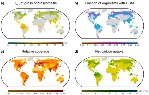
Fig. A1.Global maps of model estimates based on time averages of the last 100 yr of a 2000-yr run with 3000 initial strategies. The estimates shown in(a–d)to are based on the maximum-weighting method while the ones shown in Fig. 5 are based on the average-weighting method. Areas where no strategy has been able to survive are shaded in grey.
a) b)
c) d)
Toptof gross photosynthesis
5 10 15 20 25 30 35 40 [°C]
Fraction of organisms with CCM
0.00 0.12 0.25 0.38 0.50 0.62 0.75 0.88 1.00 [ ]
Relative coverage
0.00 0.12 0.25 0.38 0.50 0.62 0.75 0.88 1.00 [ ]
Net carbon uptake
0 2 4 6 8 10 12 14 16 [(g C) m−2yr−1]
Appendix B
Model details
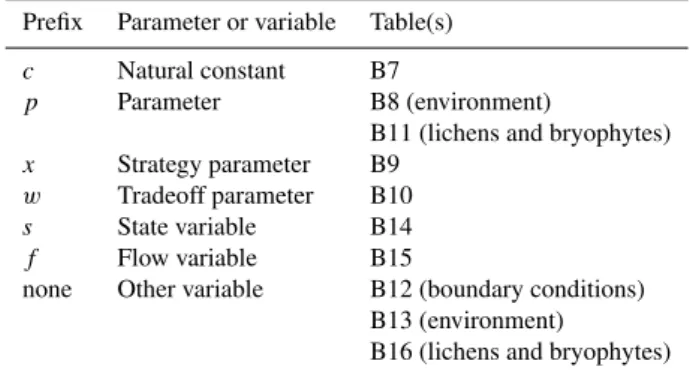
In the following sections, the technical details of the model are explained. Section B1 describes how strategies are gen-erated from parameter ranges. Moreover, references are pro-vided for these parameter ranges. Sections B2 to B7 contain all model equations that are associated with physiological processes of lichens and bryophytes. Furthermore, references are given for the theoretical background and the parameter-isation of the equations. The equations are ordered accord-ing to the structure of Sect. 2. The values and the units of the parameters and variables used in the model equations are tabulated in Tables B7 to B16. The tables contain references to the respective equations. To make the equations more eas-ily readable, characteristic prefixes are added to the model parameters and the associated tables are structured accord-ingly. The prefixes, the type of parameter and the associated table(s) can be found in Table B1.
For further details on the implementation of parameters and equations in the model, we refer to the source code of the model, which is available on request.
B1 Generation of strategies
To account for the large functional variability of lichens and bryophytes, many strategies are generated in the model, which differ from each other in 15 characteristic parameters (see Sect. 2.2). To create the strategies, these 15 characteristic parameters are assigned through randomly sampling ranges of possible values. The parameters and the corresponding ranges are listed in Table B9. Assignment of parameter val-ues is performed in two steps: (a) for each strategy, a set of 15 random numbers uniformly distributed between 0 and 1 is sampled. The random numbers are generated by a Latin Hypercube algorithm (McKay et al., 1979). This facilitates an even sampling of the 15-dimensional space of random numbers, since the space is partitioned into equal subvol-umes from which the random numbers are then sampled. (b) The 15 random numbers are then mapped to values from the ranges of the parameters. Since the purpose of the sampling is to represent the whole range of a parameter as evenly as possible, two different mapping methods are used, a linear one for parameters that have only a small range of possible values, and an exponential one for parameters that span more than one order of magnitude.
If the possible values of a parameter x span a relatively small range, a random number between 0 and 1 is linearly mapped to this range according to
x=N (xmax−xmin)+xmin (B1)
whereNis a random number between 0 and 1.xmaxandxmin are the maximum and the minimum value from the range of possible values for the parameter x. To ensure that the
ranges are sufficiently broad, more extreme values than those found in the literature are used as limits. For this purpose, the mean of the literature-based parameter values is computed. xmin is then calculated by subtracting the distance between the mean and the lowest value found in the literature from this lowest value.xmaxis calculated by adding the distance between mean and highest value found in the literature to this highest value. A precondition for this procedure is that the parameter values span a relatively small range, as mentioned above. Otherwise, subtracting the above mentioned distance from the mean would result in negative values.
If the possible values of a parameter span a large range, the mapping from a random number between 0 and 1 to this range is exponential and written as
x=xmineNlog
xmax
xmin
(B2) where the symbols have the same meaning as in Eq. (B1). The exponential function is used to represent each order of magnitude of the range equally. If the limits of the range were 1 and 10000, for instance, using Eq. (B1) would result in 90 % of the values lying between 1000 and 10000. Hence, values from the range 1 to 1000 would be strongly under rep-resented. By using Eq. (B2) this problem is avoided, which is particularly important if the model is run with low numbers of strategies. In this case, the under-representation of strate-gies with parameter values from the lower end of the range could lead to unrealistic model results. To be consistent with the exponential mapping, the limits of the range are also cal-culated differently than for Eq. (B1):xminis assumed to be half the lowest value found in the literature, whilexmaxis set to the double of the highest value found in the literature.
Additionally, random numbers can be transformed into categorical values. This is done by assigning a lichen or bryophyte to a certain category if the corresponding random number is below a threshold, and otherwise to another cate-gory. The threshold is a number between 0 and 1.
In the following, each of the 15 strategy parameters is shortly described together with references for the range of possible values.
B1.1 Albedo
The albedo xα of a lichen or bryophyte is assumed to vary from 0 to 1. The reason for this assumption is that lichens and bryophytes show a large variety of colours and therefore a large range of possible values for the albedo (Kershaw, 1975). For simplicity, each strategy has a fixed value ofxα. In reality, species can adapt their albedo to dif-ferent environmental conditions. This can be represented in the model by strategies differing only in the value ofxα.
Table B1.Overview of the nomenclature of parameters and vari-ables in the model.
Prefix Parameter or variable Table(s)
c Natural constant B7
p Parameter B8 (environment)
B11 (lichens and bryophytes)
x Strategy parameter B9
w Tradeoff parameter B10
s State variable B14
f Flow variable B15
none Other variable B12 (boundary conditions)
B13 (environment)
B16 (lichens and bryophytes)
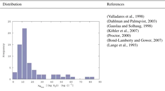
B1.2 Specific water storage capacity
The specific water storage capacityx2maxrepresents the
max-imum amount of water per gram carbon a lichen or bryophyte can store (Fig. B1). An exponential mapping is used for the range of possible values.
B1.3 Specific projected area
The specific projected areaxAspecrepresents the surface area
per gram carbon of a lichen or bryophyte projected onto a plane (Fig. B2). An exponential mapping is used for the range of possible values.
B1.4 Location of growth
The location of growthxlocof a lichen or bryophyte is a cat-egorical variable. Two categories are possible: canopy and ground. Since no data could be found about the relative abun-dance of lichens and bryophytes living in the canopy and the ones living on the ground, the probability for each location of growth is 50 %.
B1.5 Threshold saturation and shape of water potential
curve
As described in Sect. 2.1.2, the water potential9H2Ois an
in-creasing function of the water saturation of the thallus,82, which is described below in Sect. B3.1.9H2Ohas a value of
−∞at zero water content and reaches a maximum value of 0
at a certain threshold saturation (see Fig. B3). This threshold saturation represents the partitioning between water stored in the cells of the thallus and extracellular water. It is de-scribed by the parameter x82,sat. The theoretical limits of
x82,sat are 0 and 1, where 0 would mean that the lichen or
bryophyte stores all its water extracellularly and 1 would mean that no extracellular storage capacity exists. A lower limit of 0 is physiologically unrealistic. Some mosses have, however, a relatively large capacity to store water extracel-lularly (Proctor, 2000). Hence, the lower limit ofx82,sat is
set to 0.3 An upper limit of 1.0 seems realistic since
signif-icant amounts of extracellular water do not seem to occur in many lichens under natural conditions (Nash III, 1996, p. 161). Due to the small range of possible values forx82,sat, a
linear mapping is used for this parameter.
A second parameter,x9H2O, determines the shape of the water potential curve from zero water content to the thresh-old saturation. Given a certain value ofx82,sat, the parameter
x9H2Ocontrols the water content of the thallus in equilibrium with a certain atmospheric vapour pressure deficit. Since the range of possible values ofx9H2O is quite limited, a linear mapping is used. The limits for this range are estimated us-ing the data points in Fig. B3 and are set to 5.0 and 25.0, respectively. The calculation of the water potential9H2Ois
given below in Sect. B3.3.
Furthermore, the relation between water content and wa-ter potential influences the tradeoff between CO2diffusivity and metabolic activity. This is explained in detail below in Sect. B3.5.
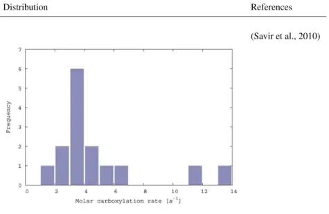
B1.6 Molar carboxylation rate of Rubisco
The molar carboxylation rate of RubiscoxVC,max represents
the maximum carboxylation velocity of a Rubisco molecule (Fig. B4). The data are taken from a study that analyses a broad range of photoautotrophs. An exponential mapping is used for the range of possible values.
B1.7 Molar oxygenation rate of Rubisco
The molar oxygenation rate of RubiscoxVO,maxrepresents the
maximum oxygenation velocity of a Rubisco molecule (Fig. B5). The data are taken from a study that analyses a broad range of photoautotrophs. A linear mapping is used for the range of possible values.
B1.8 Reference maintenance respiration rate andQ10
value of respiration
The specific respiration rate of lichens and bryophytes,Rspec, is controlled by two parameters: the reference respiration rate at 10◦C,x
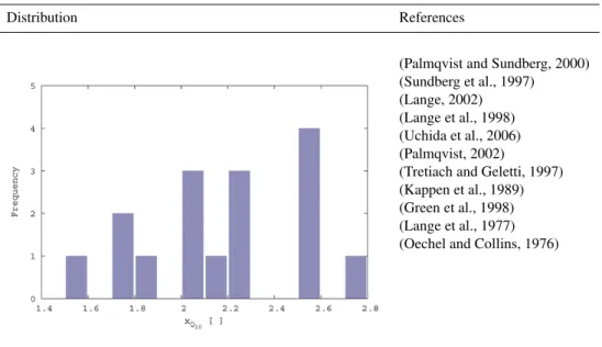
Rref; and the Q10 value of respiration, xQ10. The
distributions of these parameters are shown in Figs. B6 and B7. ForxRref an exponential mapping is used while forxQ10
a linear mapping is used. The limits ofxQ10 are not
calcu-lated by the method described for Eq. (B1) since the result-ing range would be physiologically unrealistic. Instead, the values were rounded to the nearest integer. The influences of the two parameters on respiration rate are shown in Fig. B8.