Free vibration of thick orthotropic plates using trigonometric
shear deformation theory
Abstract
In this paper a trigonometric shear deformation theory is presented for the free vibration of thick orthotropic square and rectangular plates. In this displacement based theory the in-plane displacement field uses sinusoidal function in terms of thickness coordinate to include the shear deforma-tion effect. The cosine funcdeforma-tion in terms of thickness coordi-nate is used in transverse displacement to include the effect of transverse normal strain. The most important feature of the theory is that the transverse shear stress can be ob-tained directly from the constitutive relations satisfying the shear stress free surface conditions on the top and bottom surfaces of the plate. Hence the theory obviates the need of shear correction factor. Governing equations and bound-ary conditions of the theory are obtained using the principle of virtual work. Results obtained for frequency of bending mode, shear mode and thickness stretch mode of free vibra-tion of simply supported orthotropic square and rectangular plates are compared with those of other refined theories and exact solution from theory of elasticity wherever applicable.
Keywords
shear deformation, thick orthotropic plate, transverse nor-mal strain, free vibration, frequencies.
Y. M. Ghugal∗and A. S. Sayyad Department of Applied Mechanics, Govern-ment Engineering College,
Aurangabad-431005, Maharashtra State, India
Received 06 Nov 2010; In revised form 17 May 2011
∗Author email: [email protected]
1 INTRODUCTION
The use of composite materials has increased steadily during last two decades, particularly in aerospace, underwater and automotive structures. This is largely because many compos-ite materials exhibit high strength-to-weight and stiffness-to-weight ratios, which make them ideally suited for use in weight-sensitive structures.
is limited to only thin plates; as a consequence it under predicts deflections and over predicts natural frequencies.
First order shear deformation theories (FSDTs) can be considered as improvements over classical plate theory. It is based on the assumption that straight lines normal to undeformed midplane remain straight but not necessarily normal to the deformed midplane. Mindlinet al. [18] investigated the free flexural vibration of rectangular plate. Reissner [24] was the first to develop a theory which incorporates the effect of shear. Reissner’s formulation comes out as a special case of Librescu’s [14] approach.
Chladni [3] studied the free vibration of a square plate with completely free edges. Rayleigh [22] presented his well-known general method of solution for the natural frequencies of vibra-tion. Ritz [25] improved the Rayleigh procedure by assuming a set of admissible trial functions. Levinson [12] has developed a displacement based theory which does not require shear correc-tion factor. The governing equacorrec-tions for the mocorrec-tion of a plate obtained by Levinson’s approach are same as those by Mindlin’s theory, provided that the shear coefficient value associated with the Mindlin’s theory is taken as 5/6.
Many higher order theories are available in the literature for the static flexure and free vibration analysis of thick plates e.g., theories by Nelson and Lorch [20] with nine unknowns, Krishna Murty [19] with 5, 7, 9. . . unknowns, Lo et al. [16, 17] with 11 unknowns, Kant [7] with six unknowns, Bhimaraddi and Stevens [2] with five unknowns, Reddy [23] with eight unknowns, Hanna and Leissa [5] with four unknowns. Srinivas et al. [27] used an exact three dimensional plate theory to study the vibration of simply supported homogenous and laminated thick rectangular plates.
Levy [13] has developed a refined theory for thick plate for the first time using sinusoidal functions in the displacement field. Stein [28] has used theory using trigonometric functions for analysis of laminated beams and plates. A critical review of the plate theories has been given by Vasil’ev [29] and Noor and Burton [21]. Whereas Liew et al. [15] surveyed plate theories particularly applied to thick plate vibration problems. A recent review paper is presented by Ghugal and Shimpi [4]. Shimpi and Patel [26] have developed a two variable refined plate theory for the free vibration of orthotropic plate; however theory overestimates the results of bending frequencies compared to those of exact theory. Kim and Reddy [8] have developed novel mixed finite element models for nonlinear analysis of plates based on the classical and first order shear deformation theories.
In this paper a displacement based trigonometric shear deformation theory is presented for the free vibration of orthotropic square and rectangular plates which includes effect of transverse shear and transverse normal strain.
2 PLATE UNDER CONSIDERATION
Consider a plate (of length a, width b, and thickness h) of homogenous material. The plate occupies (in O – x – y – z right-handed Cartesian coordinate system) a region
2.1 Assumptions made in theoretical formulation
1. The displacement components u and v are the inplane displacements in x and y – directions respectively and w is the transverse displacement in z-direction. These dis-placements are small in comparison with the plate thickness.
2. The in-plane displacement u in x -direction and v in y -direction each consist of two parts:
a. a displacement component analogous to displacement in classical plate theory of bending;
b. displacement component due to shear deformation which is assumed to be sinusoidal in nature with respect to thickness coordinate.
3. The transverse displacementw in z -direction is assumed to be a function ofx, y and z
coordinates.
4. The body forces are ignored in the analysis.
5. The plate is subjected to transverse load only.
2.2 The displacement field
Based upon the before mentioned assumptions, the displacement field of the present plate theory is given as below:
u(x,y,z, t)=−z∂w(x,y,t)
∂x + h πsin
π z
h ϕ(x,y,t)
v(x,y, z,t)=−z∂w(x,y,t)
∂y + h πsin
π z
h ψ(x,y,t)
w(x,y, z,t)=w(x,y,t)+h
πcos π z
h ξ(x,y,t)
(2)
where uandv are the inplane displacements in x and y –directions respectively and w is transverse displacement in z -direction. The sinusoidal function is assigned according to the shear stress distribution through the thickness of the plate. Theϕ,ψandξ represent rotations of the plate at neutral surface, which are unknown functions to be determined.
2.3 Strain displacement relationship
Normal strains:
εx = ∂u ∂x =−z
∂2
w ∂x2 +
h π sin πz h ∂ϕ ∂x
εy= ∂v ∂y =−z
∂2
w ∂y2 +
h πsin πz h ∂ψ ∂y
εz = ∂w
∂z =−ξsin πz
h
(3)
Shear strains:
γxy = ∂u ∂x+
∂v ∂x =−2z
∂2 w ∂x∂y+ h πsin πz h ( ∂ϕ ∂y + ∂ψ ∂x)
γxz= ∂u ∂z +
∂w ∂x =cos
πz h (
h π
∂ξ ∂x+ϕ)
γyz = ∂v ∂z +
∂w ∂y =cos
πz h (
h π
∂ξ ∂y+ψ)
(4)
2.4 Stress-strain relationship
The following stress-strain relationships are used to obtain normal and transverse shear stresses.
⎧⎪⎪⎪⎪ ⎪⎪⎪⎪⎪ ⎪⎪ ⎨⎪⎪⎪ ⎪⎪⎪⎪⎪ ⎪⎪⎪⎩ σx σy σz τxy τyz τzx ⎫⎪⎪⎪⎪ ⎪⎪⎪⎪⎪ ⎪⎪ ⎬⎪⎪⎪ ⎪⎪⎪⎪⎪ ⎪⎪⎪⎭ = ⎡⎢ ⎢⎢ ⎢⎢ ⎢⎢ ⎢⎢ ⎢⎢ ⎢⎣ ¯
Q11 Q¯12 Q¯13 0 0 0
¯
Q12 Q¯22 Q¯23 0 0 0
¯
Q13 Q¯23 Q¯33 0 0 0
0 0 0 Q¯44 0 0
0 0 0 0 Q¯55 0
0 0 0 0 0 Q¯66
⎤⎥ ⎥⎥ ⎥⎥ ⎥⎥ ⎥⎥ ⎥⎥ ⎥⎦ ⎧⎪⎪⎪⎪ ⎪⎪⎪⎪⎪ ⎪⎪ ⎨⎪⎪⎪ ⎪⎪⎪⎪⎪ ⎪⎪⎪⎩ εx εy εz γxy γyz γzx ⎫⎪⎪⎪⎪ ⎪⎪⎪⎪⎪ ⎪⎪ ⎬⎪⎪⎪ ⎪⎪⎪⎪⎪ ⎪⎪⎪⎭ (5)
where [Q¯ij] are the reduced stiffness coefficients as given by Jones [6] are as follows.
∆=1−µ12µ21−µ23µ32−µ31µ13−2µ21µ32µ13
¯ Q11=
E1(1−µ23µ32)
∆ ; Q¯12=
E1(µ21−µ31µ23)
∆ ;
¯ Q13=
E1(µ31−µ21µ32)
∆ ; Q¯22=
E2(1−µ13µ31)
∆ ;
¯ Q23=
E2(µ32−µ12µ31)
∆ ; Q¯33=
E3(1−µ12µ21)
∆ ;
¯
2.5 Derivation of governing equations and boundary conditions
Using Eq. (3) through (5) and dynamic version of principle of virtual work, variationally consistent differential equations and boundary conditions for the plate under consideration are obtained. The dynamic version of principle of virtual work when applied to the plate leads to:
∫zz=h/2 =−h/2 ∫
y=b
y=0 ∫ x=a
x=0
[ σxδεx+σyδεy+σzδεz
+τyzδγyz+τzxδγzx+τxyδγxy ]
dx dy dz−∫
y=b
y=0 ∫ x=a
x=0
q(x, y)δw dx dy
+ρ∫
z=h/2
z=−h/2 ∫ y=b
y=0 ∫ x=a
x=0
[∂∂t2u2 δu+
∂2
v ∂t2 δv+
∂2
w
∂t2 δw]dx dy dz=0
(6)
Employing Green’s theorem in Eq. (6) successively, we obtain the coupled Euler-Lagrange governing equations of the plate and the associated boundary conditions of the plate in terms of stress resultants. The governing differential equations are as follows:
∂2 Mx ∂x2 + 2
∂2 Mxy ∂x∂y +
∂2 My
∂y2 +q = I1 ∂2
w ∂ t2 −I2(
∂4 w ∂x2
∂t2+ ∂4
w ∂y2
∂t2)+Is1( ∂3
ϕ ∂x∂t2+
∂3 ψ
∂y∂t2)+Ic1 ∂2
ξ ∂t2 ∂Msx
∂x + ∂Vsxy
∂y − π
hVsx = Is2 ∂2
ϕ ∂t2 −Is1
∂3 w ∂x∂t2 ∂Msy
∂y + ∂Vsxy
∂x − π
hVsy=Is2 ∂2
ψ ∂t2 −Is1
∂3 w ∂y∂t2 ∂Vsx
∂x + ∂Vsy
∂y − π
hVsz=Ic1 ∂2
w ∂t2 +Ic2
∂2 ξ
∂t2 (7)
The boundary conditions at x=0 and x=aobtained are of the following form:
Mx=0 or ∂w/∂x is specified ∂Mx/∂x+2∂Mxy/∂y=0 or w is specified Msx=0 or ϕ is specified Vsxy=0 or ψ is specified Vsx=0 or ξ is specified
⎫⎪⎪⎪⎪ ⎪⎪⎪⎪ ⎬⎪⎪⎪ ⎪⎪⎪⎪⎪ ⎭
(8)
and along y=0 and y=bedges, the boundary conditions are as follows:
My=0 or ∂w/∂y is specified ∂My/∂y+2∂Mxy/∂x=0 or wis specified Msy=0 or ϕis specified
Vsxy=0 or ψis specified Vsy=0 or ξ is specified
⎫⎪⎪⎪⎪ ⎪⎪⎪⎪ ⎬⎪⎪⎪ ⎪⎪⎪⎪⎪ ⎭
(9)
At corners (x=0, y=0),(x=a, y=0),(x=0, y=b),(x=a, y=b) boundary condition is:
Here the stress resultants appear in the governing equations and boundary conditions are defined as follows:
⎡⎢ ⎢⎢ ⎢⎢ ⎢⎢ ⎣
Mx Msx My Msy Mxy Vsxy 0 Vsz
⎤⎥ ⎥⎥ ⎥⎥ ⎥⎥ ⎦ = ∫
h/2
−h/2
⎧⎪⎪⎪⎪ ⎪⎪ ⎨⎪⎪⎪ ⎪⎪⎪⎩ σx σy τxy σz ⎫⎪⎪⎪⎪ ⎪⎪ ⎬⎪⎪⎪ ⎪⎪⎪⎭ ( z h πsin πz
h )dz (11)
[ Vsx
Vsy ] = ∫ h/2
−h/2 {
τzx τzy } (
h πcos
πz
h )dz (12)
where Mx, My, Mxy are moment resultants analogous to classical plate theory, Msx, Msy are refined moments due to transverse shear deformation effect and Vsz, Vsxy, Vsx, Vsy are shear force resultants. The inertia terms appeared in the governing equations and boundary conditions are expressed as follows:
⎡⎢ ⎢⎢ ⎢⎢ ⎢⎢ ⎢⎢ ⎢⎢ ⎢⎣ I1 I2 Is1 Is2 Ic1 Ic2 ⎤⎥ ⎥⎥ ⎥⎥ ⎥⎥ ⎥⎥ ⎥⎥ ⎥⎦
=ρ∫
h/2
−h/2{1
z2 zh πsin
πz h
h2
π2sin 2πz h h πcos πz h h2
π2cos 2πz
h }dz (13)
3 ILLUSTRATIVE EXAMPLES
Simply supported orthotropic square and rectangular plates occupying the region given by the Eqn. (1) are considered for numerical study. The governing differential equations (7) and the associated boundary conditions (8 and 9), in terms of displacement variables, for free vibration of square and rectangular plates under consideration are as follows:
(D1
∂4
w ∂x4 +D2
∂4
w ∂x2∂y2+D3
∂4
w
∂y4)−(D4
∂3
ϕ ∂x3 +D5
∂3
ψ
∂y3)−D6(
∂3
ϕ ∂x∂y2 +
∂3
ψ
∂x2∂y)+D7
∂2
ξ ∂x2
+D8
∂2
ξ ∂y2+I1
∂2
w ∂ t2 −I2(
∂4
w ∂x2∂t2 +
∂4
w
∂y2∂t2) +Is1(
∂3
ϕ ∂x∂t2+
∂3
ψ
∂y∂t2)+Ic1
∂2
ξ ∂t2 =q
(14)
D4
∂3
w ∂x3 +D6
∂3
w ∂x∂y2−D9
∂2
ϕ ∂x2 −D10
∂2
ϕ
∂y2 +D11ϕ−D12
∂2
ψ ∂x∂y+D13
∂ξ ∂x+Is2
∂2
ϕ ∂t2 −Is1
∂3
w ∂x∂t2 =0
(15)
D5
∂3w ∂y3 +D6
∂3w
∂x2∂y −D10
∂2ψ ∂x2 −D14
∂2ψ
∂y2 +D15ψ−D12
∂2ϕ ∂x∂y+D16
∂ξ ∂y+Is2
∂2ψ ∂t2 −Is1
∂3w ∂y∂t2 =0
D7
∂2
w ∂x2 +D8
∂2
w ∂y2 −D13
∂ϕ ∂x −D16
∂ψ
∂y −(D17 ∂2
ξ ∂x2+D18
∂2
ξ
∂y2+D19ξ)+Ic1
∂2
w ∂t2 +Ic2
∂2
ξ ∂t2 =0
(17) The associated boundary conditions on edges x=0 and x=aare as follows:
w=0 (18)
D1
∂2w ∂x2 +D21
∂2w ∂y2 −D4
∂ϕ ∂x−D22
∂ψ
∂y +D7ξ=0 (19)
D4
∂2w ∂x2 +D22
∂2w ∂y2 −D9
∂ϕ ∂x −D23
∂ψ
∂y +D24ξ=0 (20)
D20
∂2w
∂x∂y −D10( ∂ϕ ∂y +
∂ψ
∂x)=0 (21)
D25ϕ+D17
∂ξ
∂x =0 (22)
The associated boundary conditions on edges y=0 andy=b are as follows:
w=0 (23)
D21
∂2w ∂x2 +D3
∂2w ∂y2 −D22
∂ϕ ∂x −D5
∂ψ
∂y +D8ξ=0 (24)
D20
∂2w
∂x∂y +D10( ∂ϕ ∂y +
∂ψ
∂x)=0 (25)
D22
∂2
w ∂x2 +D5
∂2
w ∂y2 −D23
∂ϕ ∂x−D14
∂ψ
∂y +D26ξ=0 (26)
D27ψ+D18
∂ξ
∂y =0 (27)
3.1 The solution scheme
The governing equations for free flexural vibration of orthotropic plate can be obtained by setting the applied transverse load equal to zero in Eq. (14). A solution to resulting governing equations, when expressed in terms of displacement variables, which satisfies the associated boundary conditions (time dependent), is of the following form:
w(x, y)=
m=∞ ∑
m=1
n=∞ ∑
n=1
wmnsin mπx
a sin nπy
b sinωmnt
ϕ(x, y)=
m=∞ ∑
m=1
n=∞ ∑
n=1
ϕmncos mπx
a sin nπy
b sinωmnt
ψ(x, y)=
m=∞ ∑
m=1
n=∞ ∑
n=1
ψmnsin mπx
a cos nπy
b sinωmnt
ξ(x, y)=
m=∞ ∑
m=1
n=∞ ∑
n=1
ξmnsin mπx
a sin nπy
b sinωmnt
(28)
where wmn is the amplitude of translation and ϕmn, ψmn and ξmn are the amplitudes of rotation. ωmn is the natural frequency of mth and nth mode of vibration. Substitution of solution form given by Eqn. (28) into the governing equations (14-17) of free vibration of orthotropic plate results in following algebraic equations:
⎡⎢ ⎢⎢ ⎢⎣
(D1m
4 π4 a4 +D2
m2n2π4 a2b2 +D3
n4π4
b4 )wmn−(D4 m3π3
a3 +D6 mn2π3
ab2 )ϕmn −(D5n
3 π3
b3 +D6m
2 nπ3
a2b )ψmn−(D7m
2 π2 a2 +D8n
2 π2 b2 )ξmn
⎤⎥ ⎥⎥ ⎥⎦− ω
2
[(I1+I2
m2π2 a2 +I2
n2π2
b2 )wmn− Is1
mπ
a ϕmn−Is1 nπ
b ψmn+Ic1ξmn]=0
(29)
⎡⎢ ⎢⎢ ⎢⎣
(D4m
3 π3
a3 +D6mn
2 π3
ab2 )wmn−(D9m
2 π2
a2 +D10n
2 π2
b2 +D11)ϕmn
+D12mnπ
2
ab ψmn−D13 mπ
a ξmn
⎤⎥ ⎥⎥ ⎥⎦−ω
2
[−Is1
mπ
a wmn+Is2ϕmn]=0
(30)
⎡⎢ ⎢⎢ ⎢⎣
(D5n
3 π3 b3 +D6
m2nπ3
a2b )wmn+D12 mnπ2
ab ϕmn
−(D10m
2 π2
a2 +D14n
2 π2
b2 +D15)ψmn−D16nπb ξmn ⎤⎥ ⎥⎥ ⎥⎦−ω
2
[−Is1
nπ
b wmn+Is2ψmn]=0 (31)
⎡⎢ ⎢⎢ ⎢⎣
(D7m
2 π2 a2 +D8n
2 π2
a2 )wmn−D13mπa ϕmn−D16nπb ψmn −(D17m
2 π2
a2 +D18n
2 π2
a2 +D19)ξmn
⎤⎥ ⎥⎥ ⎥⎦−ω
2
Equations (29) through (32) can be written in the following matrix form:
⎛ ⎜⎜ ⎜⎜ ⎝ ⎡⎢ ⎢⎢ ⎢⎢ ⎢⎢ ⎣
K11 K12 K13 K14
K21 K22 K23 K24
K31 K32 K33 K34
K41 K42 K43 K44
⎤⎥ ⎥⎥ ⎥⎥ ⎥⎥ ⎦
−ω2 ⎡⎢ ⎢⎢ ⎢⎢ ⎢⎢ ⎣
M11 M12 M13 M14
M21 M22 M23 M24
M31 M32 M33 M34
M41 M42 M43 M44
⎤⎥ ⎥⎥ ⎥⎥ ⎥⎥ ⎦
⎞ ⎟⎟ ⎟⎟ ⎠
⎧⎪⎪⎪⎪ ⎪⎪ ⎨⎪⎪⎪ ⎪⎪⎪⎩
wmn ϕmn ψmn ξmn
⎫⎪⎪⎪⎪ ⎪⎪ ⎬⎪⎪⎪ ⎪⎪⎪⎭
= 0
(33) Eqn. (33) in more compact form can be written as follows:
([K] − ωmn2 [M]) {∆mn}= 0 (34) where[K]is the stiffness matrix,[M]is the mass matrix and{∆mn}is the vector of amplitudes of translation and rotations. The solution of Eqn. (34) is well known (see Bathe [1]), from this solution lowest natural frequencies for all modes of vibration can be obtained. The orthotropic plate has following material properties as given by Srinivas et al. [27]:
¯
Q11=23.2×10⁶psi, Q¯22=12.6×10⁶psi, Q¯33=12.3×10⁶psi,
¯
Q12=5.41×10 6
psi, Q¯13=0.25×10 6
psi, Q¯23=2.28×10 6
psi, ¯
Q44=6.19×10 6
psi, Q¯55=3.71×10 6
psi, Q¯66=6.10×10 6
psi.
The density (ρ) of material can be taken as any arbitrary value for calculation of frequencies.
4 NUMERICAL RESULTS
In the present paper free vibration analysis of simply supported square and rectangular or-thotropic plate for aspect ratio 10 is attempted. The results obtained using present theory are compared with exact results and those of other higher order theory results available in litera-ture wherever applicable. Following non-dimensional form is used for the purpose of presenting the results in this paper.
¯
ω=ωmnh
√ ρ Q11
The percentage error in the results obtained using a particular model with respect to the results of exact elasticity solutions is calculated as follows:
%error= value by perticular theory−value by exact elasticity solution
value by exact elasticity solution ×100
4.1 Discussion of numerical results
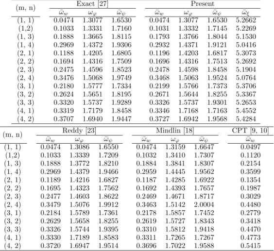
Table 1 Comparison of natural frequencies of orthotropic square plate (b/a=1) for aspect ratio 10 (h/a=0.1).
(m, n) Exact [27] Present
¯
ωw ωϕ ω¯ψ ω¯w ωϕ ω¯ψ ω¯ξ
(1, 1) 0.0474 1.3077 1.6530 0.0474 1.3077 1.6530 5.2662 (1,2) 0.1033 1.3331 1.7160 0.1031 1.3332 1.7145 5.2269 (1, 3) 0.1888 1.3665 1.8115 0.1793 1.3766 1.8044 5.1530 (1, 4) 0.2969 1.4372 1.9306 0.2932 1.4371 1.9121 5.0416 (2, 1) 0.1188 1.4205 1.6805 0.1196 1.4203 1.6817 5.3073 (2, 2) 0.1694 1.4316 1.7509 0.1696 1.4316 1.7513 5.2692 (2, 3) 0.2475 1.4596 1.8523 0.2478 1.4598 1.8458 5.1904 (2, 4) 0.3476 1.5068 1.9749 0.3468 1.5063 1.9524 5.0764 (3, 1) 0.2180 1.5777 1.7334 0.2199 1.5766 1.7373 5.3706 (3, 2) 0.2624 1.5651 1.8195 0.2671 1.5644 1.8255 5.3367 (3, 3) 0.3320 1.5737 1.9289 0.3326 1.5737 1.9301 5.2653 (4, 1) 0.3319 1.7179 1.8458 0.3346 1.7168 1.7163 5.4552 (4, 2) 0.3707 1.6940 1.9447 0.3727 1.6942 1.9568 5.4284
(m, n) Reddy [23] Mindlin [18] CPT [9, 10] ¯
ωw ωϕ ωψ¯ ωw¯ ωϕ ωψ¯ ωw¯
(1, 1) 0.0474 1.3086 1.6550 0.0474 1.3159 1.6647 0.0497 (1,2) 0.1033 1.3339 1.7209 0.1032 1.3410 1.7307 0.1120 (1, 3) 0.1888 1.3772 1.8210 0.1884 1.3841 1.8307 0.2154 (1, 4) 0.2969 1.4379 1.9466 0.2959 1.4445 1.9562 0.3599 (2, 1) 0.1189 1.4216 1.6827 0.1187 1.4285 1.6922 0.1354 (2, 2) 0.1695 1.4323 1.7562 0.1692 1.4393 1.7657 0.1987 (2, 3) 0.2477 1.4603 1.8622 0.2469 1.4671 1.8717 0.3029 (2, 4) 0.3479 1.5076 1.9912 0.3463 1.5142 2.0004 0.4480 (3, 1) 0.2184 1.5789 1.7361 0.2178 1.5857 1.7452 0.2779 (3, 2) 0.2629 1.5658 1.8255 0.2619 1.5727 1.8343 0.3418 (3, 3) 0.3326 1.5744 1.9395 0.3310 1.5812 1.9418 0.4470 (4, 1) 0.3330 1.7189 1.8583 0.3311 1.7265 1.7267 0.4773 (4, 2) 0.3720 1.6947 1.9514 0.3696 1.7022 1.9588 0.5415
A) Bending frequency (ω¯w): Table 1 shows comparison of bending frequencies for all modes of vibration for square plate (b/a = 1). It can be seen from Table 1 that the present theory yields excellent values of frequencies for all modes of vibration. The present theory, Reddy’s theory [23] and Mindlin’s theory [18] predicts exact result of bending frequency for fundamental
mode i.e. m = 1, n = 1. Maximum percentage error predicted by present theory is 5.39 %
whenm = 4,n= 2 whereas maximum percentage error in Reddy’s [23] theory is 3.50 % for the same mode of vibration. The theory of Kirchhoff (CPT) [9, 10] overestimates the fundamental bending frequency by 4.85 %.
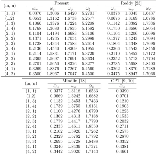
Comparison of bending frequency for the rectangular plate (b/a=√2) is shown in Table
Table 2 Comparison of natural frequencies of orthotropic rectangular plate (b/a=√2) for aspect ratio 10
(h/a= 0.1).
(m, n) Present Reddy [23]
¯
ωw ωϕ ω¯ψ ω¯ξ ω¯w ωϕ ω¯ψ
(1, 1) 0.0376 1.3036 1.6420 5.2701 0.0378 1.3045 1.6437 (1,2) 0.0653 1.3162 1.6738 5.2577 0.0676 1.3169 1.6786 (1, 3) 0.1066 1.3376 1.7224 5.2208 0.1142 1.3382 1.7336 (1, 4) 0.1768 1.3680 1.7835 5.1582 0.1750 1.3686 1.8054 (2, 1) 0.1104 1.4194 1.6683 5.3106 0.1104 1.4206 1.6696 (2, 2) 0.1371 1.4235 1.7054 5.2989 0.1377 1.4243 1.7094 (2, 3) 0.1728 1.4344 1.7583 5.2614 0.1804 1.4348 1.7696 (2, 4) 0.2136 1.4540 1.8209 5.1955 0.2366 1.4543 1.8456 (3, 1) 0.2114 1.5831 1.7171 5.3729 0.2110 1.5852 1.7172 (3, 2) 0.2365 1.5697 1.7691 5.3634 0.2352 1.5713 1.7704 (3, 3) 0.2701 1.5650 1.8326 5.3277 0.2735 1.5658 1.8400 (4, 1) 0.3269 1.8376 1.7267 5.4560 0.3262 1.8370 1.7289 (4, 2) 0.3500 1.8967 1.7047 5.4500 0.3475 1.8947 1.7066
(m, n) ¯ Mindlin [18] CPT [9, 10]
ωw ωϕ ωψ¯ ωw¯
(1, 1) 0.0377 1.3118 1.6533 0.0390 (1,2) 0.0669 1.3242 1.6882 0.0701 (1, 3) 0.1132 1.3453 1.7433 0.1210 (1, 4) 0.1739 1.3755 1.8151 0.1903 (2, 1) 0.1100 1.4276 1.6790 0.1225 (2, 2) 0.1362 1.4313 1.7188 0.1533 (2, 3) 0.1779 1.4417 1.7790 0.2032 (2, 4) 0.2333 1.4611 1.8550 0.2711 (3, 1) 0.2102 1.5920 1.7262 0.2575 (3, 2) 0.2329 1.5782 1.7792 0.2870 (3, 3) 0.2695 1.5728 1.8488 0.3352 (4, 1) 0.3246 1.8439 1.7371 0.4381 (4, 2) 0.3442 1.9020 1.7143 0.4661
theories due to the neglect of transverse shear deformation and transverse normal stress effects in the classical theory.
B) Thickness shear mode frequency (¯ωϕ): From the examination of Table 1 it can be
observed that, for square plate (b/a = 1) the present theory gives exact values of thickness shear mode frequency for fundamental mode of vibrationi.e. m = 1, n = 1 whereas theories of Reddy [23] and Mindlin [18] overestimates the same by 0.069 % and 0.63 % respectively for the same mode of vibration as compared to that of exact theory. The present theory yield excellent results for the thickness shear mode frequency for all higher modes of vibration. The theories of Reddy [23] and Mindlin [18] show higher values for the thickness shear mode frequency for all modes of vibration as compared to those of exact and present theory. The comparison of thickness shear mode frequency for rectangular plate (b/a = √2) as shown in
more or less identical with each other. However, Mindlin’s [18] theory predicts higher values of this frequency.
Dynamic shear correction factor is the most important parameter in the dynamic analysis of plates. The exact value of this factor is given by Lamb [11]. Present theory yields the exact value of dynamic shear correction factor (π2
/12) from the circular frequency of thickness shear motion (m = 0, n = 0) for infinitely long thin rectangular plate.
C) Thickness shear mode frequency (ω¯ψ): From Table 1 it is observed that, for square plate (b/a = 1) present theory predicts exact result of this frequency for fundamental mode whereas Reddy [23] and Mindlin [18] theories overestimate the same. The theories of Reddy [23] and Mindlin [18] shows less accuracy of results for higher modes as compared to those of present and exact theories. The comparison of frequency of thickness shear mode for rectangular plate (b/a=√2) is shown in Table 2.
D) Thickness stretch mode frequency (¯ωξ): In Table 1 and 2 results of frequency of thickness stretch mode of vibration are given for square and rectangular plates. The results of this frequency by other higher order theories are not available in the literature due to the neglect of transverse normal strain effect in these theories. The lowest natural frequency for this mode occurs at m = 1 and n = 4 and the highest natural frequency occurs at m = 4 and n = 1.
5 CONCLUSIONS
Following conclusions are drawn from the free vibration analysis thick orthotropic plates using variationally consistent trigonometric shear deformation theory.
1. The frequencies obtained by the present theory for bending and thickness shear modes of vibration for all modes of vibration are in excellent agreement with the exact values of frequencies for the square plate (b/a = 1).
2. The frequencies of bending and thickness shear modes of vibration according to present theory are in good agreement with those of higher order shear deformation theory for rectangular plate (b/a=√2) and these results are rarely available in the literature.
3. The present theory is capable to produce frequencies of thickness stretch mode of vibra-tion.
4. The present theory yields the exact value of dynamic shear correction factor from the thickness shear motion of vibration.
References
[1] K.J. Bathe. Finite Element Procedures. Prentice Hall of India Pvt. Ltd., New Delhi, 1996.
[3] E. F. F. Chladni. Die Akustik. Leipzig, 1802.
[4] Y.M. Ghugal and R.P. Shimpi. A review of refined shear deformation theories for isotropic and anisotropic laminated plates. Journal of Reinforced Plastics and Composites, 21:775–813, 2002.
[5] N.F. Hanna and A.W. Leissa. A higher order shear deformation theory for the vibration of thick plates. Journal of Sound and Vibration, 170:545–555, 1994.
[6] R.M. Jones. Mechanics of Composite Materials. Scripta Book Co., Washington, D.C., 1975.
[7] T. Kant. Numerical analysis of thick plates. Computer methods in Applied Mechanics and engineering, 31(1):1–18, 1982.
[8] W. Kim and J.N. Reddy. Novel mixed finite element models for nonlinear analysis of plates.Latin American Journal of Solids and Structures, 7:201–226, 2010.
[9] G.R. Kirchhoff. Uber das gleichgewicht und die bewegung einer elastischen scheibe. Journal of Reine Angew. Math. (Crelle), 40(51-88), 1850.
[10] G.R. Kirchhoff. Uber die uchwingungen einer kriesformigen elastischen scheibe. Poggendorffs Annalen, 81:58–264, 1850.
[11] H. Lamb. On waves in an elastic plate. InProceedings of the Royal Society of London, volume 93, pages 114–128, England, 1917. Series A.
[12] M. Levinson. An accurate, simple theory of the statics and dynamics of elastic plates. Mechanics: Research Com-munications, 7:343–350, 1980.
[13] M. Levy. Memoire sur la theorie des plaques elastique planes. Journal des Mathematiques Pures et Appliquees, 30:219–306, 1877.
[14] L. Librescu. Elastostatic and Kinetics of anisotropic and Heterogeneous shell-Type structures. Noordhoff Interna-tional, Leyden, The Netherlands, 1975.
[15] K.M. Liew, Y. Xiang, and S. Kitipornchai. Research on thick plate vibration: a literature survey.Journal of Sound and Vibration, 180:163–176, 1995.
[16] K.H. Lo, R.M. Christensen, and E.M. Wu. A high-order theory of plate deformation, Part 1: homogeneous plates.
ASME Journal of Applied Mechanics, 44:663–668, 1977.
[17] K.H. Lo, R.M. Christensen, and E.M. Wu. A high-order theory of plate deformation, Part 2: Laminated plates.
ASME Journal of Applied Mechanics, 44:669–676, 1977.
[18] R.D. Mindlin. Influence of rotatory inertia and shear on flexural motions of isotropic, elastic plates. ASME Journal of Applied Mechanics, 18:31–38, 1951.
[19] A.V. Krishna Murty. Higher order theory for vibrations of thick plates. AIAA Journal, 15(12):1823–1824, 1977.
[20] R.B. Nelson and D.R. Lorch. A refined theory for laminated orthotropic plates.ASME Journal of Applied Mechanics, 41:177–183, 1974.
[21] A.K. Noor and W.S. Burton. Assessment of shear deformation theories for multilayered composite plates. Applied Mechanics Reviews, 42:1–13, 1989.
[22] L. Rayleigh. Theory of sound, volume I. Macmillan, London, 1877. reprinted 1945 by Dover, New York.
[23] J.N. Reddy. A refined nonlinear theory of plates with transverse shear deformation. International Journal of Solids and Structures, 20(9/10):881–896, 1984.
[24] E. Reissner. The effect of transverse shear deformation on the bending of elastic plates. ASME Journal of Applied Mechanics, 12:69–77, 1945.
[25] W. Ritz. Uber eine neue method zur losung gewisser variations problem der mathematischen physic. Journal fur Reine und Angewandte Mathematik, 135:1–161, 1909.
[26] R.P. Shimpi and H.G. Patel. A two variable refined plate theory for orthotropic plate analysis.International Journal of Solids and Structures, 43:6783–6799, 2006.
[28] M. Stein and N.J.C. Bains. Post buckling behavior of longitudinally compressed orthotropic plates with transverse shearing flexibility.AIAA Journal, 28:892–895, 1990.
APPENDIX
The stiffness coefficientsD1throughD27appeared in governing equations (14-17) and
bound-ary conditions (18-27) are as follows.
D1= ¯
Q11h 3
12 ;D2=2(Q¯12+2 ¯Q66)
h3
12;D3= ¯
Q22h 3
12 ;D4= ¯
Q112h 3 π3 ;D5=
¯
Q222h 3 π3 ; D6=2(Q¯12+2 ¯Q66)h
3 π3;D7=
¯
Q132h 2 π2 ;D8=
¯
Q232h 2 π2 ;D9=
¯
Q11h 3
2π2 ;D10=
¯
Q66h 3
2π2 ; D11=
¯
Q55h
2 ;D12=(Q¯12+Q¯66)
h3
2π2;D13=(Q¯13+Q¯55)h
2
2π;D14= ¯
Q22h 3
2π2 ;D15= ¯
Q44h
2 ;
D16=(Q¯23+Q¯44)h
2
2π;D17= ¯
Q55h 3
2π2 ;D18= ¯
Q44h 3
2π2 ;D19= ¯
Q33h
2 ;D20= 4 ¯Q66h
3 π3 ; D21=
¯
Q12h 3
12 ;D22= ¯
Q122h 3 π3 ;D23=
¯
Q12h 3
2π2 ;D24=
¯
Q13h 2
2π ;D25=
¯
Q55h 2
2π ;D26=
¯
Q23h 2
2π ; D27=
¯
Q44h2
2π .
The elements of stiffness matrix [K] are as under:
K11=(D1m
4 π4 a4 +D2
m2n2π4 a2b2 +D3
n4π4
b4 ); K12=(D4 m3π3
a3 +D6 mn2π3
ab2 ); K13=−(D5n
3 π3 b3 +D6
m2nπ3
a2b ); K14=−(D7 m2π2
a2 +D8 n2π2
b2 );
K21=K12; K22=−(D9
m2π2 a2 +D10
n2π2
b2 +D11); K23=D12
mnπ2
ab ; K24=−D13 mπ
a ;
K31=K13; K32=K23; K33=−(D10
m2π2 a2 +D14
n2π2
b2 +D15);K34=−D16
nπ b ;
K41=K14; K42=K24; K43=K34; K44=(D17
m2
π2
a2 +D18
n2
π2
a2 +D19)
The elements of mass matrix [M] are as under:
M11 = (I1+I2m
2 π2 a2 +I2
n2π2
b2 ); M12 = −Is1 mπ
a ; M13 = −Is1 nπ
b ; M14 = Ic1; M21 = M12; M22 = Is2; M23 = 0.0; M24 = 0.0; M31 = M13; M32 = M23;
M33 = Is2; M34 = 0.0; M41 = M14; M42 = M24; M43 = M34; M44 = Ic2.
The vector {∆mn} in Eqn. (34) is defined as: