A local-restart coupled strategy for simultaneous sizing and
geometry truss optimization
Abstract
This paper presents an approach for the global optimization of truss sizing and geometry that is based on a probabilis-tic restart procedure coupled with a local search algorithm. The resulting algorithm is able to guarantee local optimality and provides a set of local optima which contain, with an increasing probability as the number of restarts increases, the global solution. The optimization problem searches for a truss structure of minimum volume, subject to stress con-straints. The design variables are the bars cross-section areas and some nodal coordinates. Several loading conditions are also considered. Finally, four numerical examples are pre-sented and the main aspects of the approach are discussed. Keywords
global optimization, truss structures, geometry optimization, size optimization, stress constraints, minimum volume
Andr´e Jacomel Toriia,
Rafael Holdorf Lopezb and
Marco Antˆonio Luersenc,∗ a
Departamento Acadˆemico de Constru¸c˜ao Civil, Universidade Tecnol´ogica Federal do Paran´a (UTFPR), Curitiba, PR – Brazil
b
Departamento de Engenharia Civil, Universi-dade Federal de Santa Catarina (UFSC), Flo-rian´opolis, SC – Brazil
c
Laborat´orio de Mecˆanica Estrutural (LaMEs), Universidade Tecnol´ogica Federal do Paran´a (UTFPR), Curitiba, PR – Brazil
Received 18 Jan 2011; In revised form 05 May 2011
∗Author email: [email protected]
1 INTRODUCTION
The truss sizing optimization problem (where the member’s cross-sections areas are taken as design variable) can be stated, in many cases, as a Linear Programming (LP) problem [11, 16, 17]. One of the interesting characteristics of LP problems is that, when they are feasible, they always have a single global optimum or a convex set of local optima that are all global optima [15]. That is, in the case of sizing optimization problems that are stated as LP problems, every optimum solution found is indeed a global optimum.
search for global optima, and consequently, these techniques have been applied extensively to the problem studied here. However, these techniques do not guarantee local optimality [3, 5] and require, in general, a large amount of calculations [5]. Consequently, the solutions given by metaheuristics frequently present some kind of residual, such as bars that clearly do not compose an optimum solution.
Gradient based algorithms (i.e. Sequential Quadratic Programming and Interior Point Methods) were also successfully applied to the problem being addressed [2, 3, 12, 22]. These techniques are efficient for local searches and local optimality can be guaranteed [3]. That is, the solutions given by this approach do not present residuals and, in most cases, require fewer calculations than most metaheuristics. However, such techniques are not global optimization algorithms, and consequently may give poor results for problems that present several local optima.
This paper presents a local-global strategy for the simultaneous geometry and sizing opti-mization of truss structures. The optiopti-mization problem searches for a structure of minimum volume, subject to stress constraints. Local search is performed by gradient based techniques and thus local optimality is guaranteed. In order to find the global minimum, the local search is made global by a probabilistic restart procedure presented by Luersen and Le Riche [13]. In this approach, a spatial probability of starting a local search is built based on past searches. As a result, when the optimization algorithm ends, a list with several local optima (eventually the global optimum) is obtained. The proof that a local search converges to the global opti-mum for a continuous regular function when the number of random restarts goes to infinity is presented by Ritto et al. [19]. However, it should be pointed out that the restart procedure used here is not purely a random one, but it is based on information obtained from previous results, making the global search more efficient.
This paper is organized as follows. Section 2 presents the formulation of the optimization problem. The local-global optimization strategy is presented in section 3 and in the section 4, numerical examples are solved to demonstrate the strategy developed in this paper. Finally, a summary of the work and the main conclusions are presented in section 5.
2 OPTIMIZATION PROBLEM
2.1 Formulation
The truss optimization problem stated in this paper is based on the ground structure approach that is described in detail by Kocvara and Zowe [12], Achtziger [2] and Rozvany [20]. In this approach, we assume an initial truss structure composed of as many bars as needed (called the ground structure), and take as design variables the cross-section areas and some nodal coordinates of this structure. Note that bars are not included nor removed from the ground structure. However, the algorithm can reproduce the effect of removing bars from the structure by reducing its cross-section area to very small values. Computational difficulties involved in this approach are discussed in details by Cheng and Guo [7] and Stolpe and Svanberg [23].
subject to stress constraints and, as mentioned above, assuming some nodal coordinates and members cross-section areas as design variables. This optimization problem can be stated as [7]:
Find: xand A
that gives
minV(x,A)=AT.L(x), (1)
subject to
gj =Aj(σj(x,A)−σt)≤ε (j=1,2, ..., m), (2)
gj+m=Aj(σc−σj(x,A))≤ε (j=1,2, ..., m), (3)
where V is the volume of the structure, xis the vector of nodal coordinates, A is the vector of member cross-section areas, L is the vector of member lengths, gj are stress constraints,
σj is the stress on member j, σt is the allowable stress in tension (a positive value), σc is
the allowable stress in compression (a negative value), ε>0 is a small positive quantity that
is reduced during the optimization procedure and m is the number of members subjected to stress constraints.
Each stress constraint from Eq. (2) and Eq. (3) is multiplied by the cross section area of the bars in order to allow the cross section areas to be reduced to very small values without violating the constraints. When the cross section area of a given bar goes to zero, then the stress in this bar goes to infinity. Consequently, in order to allow the optimization procedure to obtain very small values for the cross section areas without violating the constraints, one must apply some constraint relaxation technique. Note that by multiplying the entire constraint by the cross section area of the bar involved, one guarantees that when the cross section area is zero the constraint will not be violated. However, this measure alone is not enough to ensure convergence of the algorithm, since during the optimization procedure the cross section areas never become zero. It is also necessary to allow the constraints to be smaller than some small quantity ε>0 instead of simply being smaller than zero during the optimization
process. These two modifications ensure that the cross section areas can be reduced to very small values without violating the constraints. The value of ε is then reduced during the optimization procedure, in order to enforce that the stresses inside the bars be smaller than the maximum allowable stresses. This strategy was first proposed by Cheng and Guo [7] and is further discussed by Stolpe and Svanberg [23].
For convenience, the design variablesAandxcan be grouped into a single design vectorX, and the constraints from Eq. (2) and Eq. (3) can be grouped into a single vector of constraints
g. In this way, the previous problem is concisely rewritten as
Find: X
that gives
min V(X)=AT.L, (4)
subject to
g(X)≤0, (5)
where g is a vector with 2m components since there are two constraints (i.e. tension and compression allowable stresses) defined for each bar of the structure. Several loading conditions can be considered by defining one vector g composed by the stress constraints of all loading conditions.
It is important to point out that the global optimization strategy proposed here is based on solving the optimization problem several times for different initial solutions, but does not depend on how these problems are solved or how these problems are formulated. Consequently, modifications to the formulation of the optimization problem do not lead to modifications on the global optimization strategy. Thus, different formulations for the truss optimization problem (considering buckling, for example) can be used without reworking on the global optimization algorithm. In this context, the formulation of the optimization problem used here is kept as simple as possible in order to allow a better understanding of the global optimization strategy. Sensitivity analysis can be made as discussed by [10], while the stresses in the bars can be obtained as discussed by [6].
2.2 Bounds on the design variables
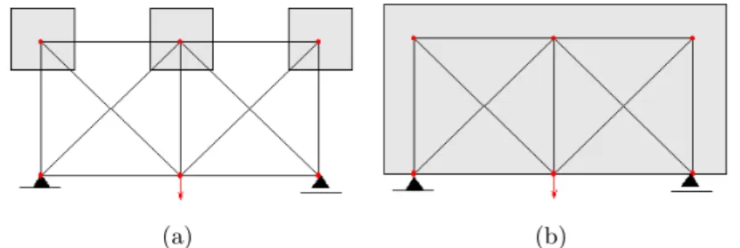
There are two different approaches for defining bounds on the nodal coordinates. In the first approach, bounds can be defined locally for each design variable, like shown in Fig. 1(a). In this case, there are different bounds for each design variable, and this can be accomplished by defining a rectangular feasible region around each node [1]. The second approach is that of defining bounds for all the design variables at once, like shown in Fig. 1(b). In this case, the bounds are the same for all design variables.
These two approaches may lead to different results, since the feasible domain defined in the first approach is smaller. However, the first approach may prevent problems related to node superposition, if the bounds are defined properly. Therefore, this approach may be rec-ommended when there are many nodes for which the coordinates are taken as design variables in the optimization procedure.
(a) (b)
Figure 1 Bounds on nodal coordinates defined (a) separately for each node, and (b) globally for all nodes.
have zero length leading to ill conditioned stiffness matrices and blocking the optimization procedure. One measure for avoiding this difficulty is by imposing bounds on nodal coordinates so that node melting is avoided, as proposed previously. However, this approach may prevent the optimization algorithm from obtaining true optimum solutions and is not recommended when very accurate solutions are sought. An elegant approach for dealing with node melting is proposed by Achtziger [3] that allows nodes to occupy the same position without blocking the optimization procedure. This approach allows one to obtain very accurate solutions, but at the cost of a modified optimization problem. A more detailed discussion on node melting is presented by Achtziger [2, 3].
For members areas, it is necessary to allow only positive values, defining in this way a lower bound for these design variables. However, in order to avoid singularity of the stiffness matrix, it is important to define a lower bound that is bigger than zero. Upper bounds on member’s areas are not strictly necessary, since the algorithm will seek a structure with minimum volume.
3 LOCAL-RESTART STRATEGY FOR GLOBAL OPTIMIZATION
As already mentioned in the introduction of this paper, the problem of geometry and sizing optimization of truss structures may present local minima that are not global minima. Under this condition, deterministic optimization algorithms such as gradient methods, Newton meth-ods or sequential simplex methmeth-ods, may not converge to the global minimum of the problem. Then, the use of a global optimization algorithm is required.
instance, reference [22]).
Here, a local-global optimization strategy, where the restart procedure uses an adaptive probability density function built using the memory of past local searches, is presented. The local search is performed using Sequential Quadratic Programming (SQP) [15], but the global optimization strategy remains unchanged if another local search algorithm is employed. The search is then turned into an asymptotically global one applying the probabilistic restart procedure proposed by Luersen and Le Riche [13].
Consider that the probability of having sampled a point X be described by a Gaussian-Parzen-window approach [9]:
P(X)= 1 N
N ∑ i=1
pi(X), (6)
whereN is the number of pointsS(i)already sampled. Such points come from the memory kept
from the previous local searches, being, in the present version of the algorithm, all the starting points and local optima already found. pi(X) is the normal multidimensional probability
density function given by:
pi(X)=
1
(2π) n
2det(Σ)12
×exp(−1
2(X−S(i))
T
Σ−1
(X−S
(i))), (7)
where n is the problem dimension (number of variables) andΣis the covariance matrix:
Σ= ⎡⎢ ⎢⎢ ⎢⎢ ⎣ σ2 1 ⋱ σ2 n ⎤⎥ ⎥⎥ ⎥⎥ ⎦ , (8)
and variances are estimated by the relation:
σj2=β(Xmax
j −X min j )
2
, (9)
where β is a positive parameter that controls the length of the Gaussians, and Xjmax and
Xmin
j are the bounds of the jth design variable. To keep the method simple, such
vari-ances are kept constant during the optimization. At the first local search, the initial point
X0 is given by the user. At the end of each local search, M points are randomly sampled
(X1,X2, . . . ,XM) and the one that minimizes Eq.(6) is selected as the initial point to restart the next local search.
The stopping criterion of the global optimization is the maximum number of local searches,
nmax, defined a priori by the user.
based techniques present good performance for finding local optima. On the other hand, the probabilistic restart explores different areas of the domain searching for the global optimum. These are important advantages over other global optimization methods, such as some heuris-tics like genetic algorithms, since the latter need, in general, much higher computational effort in order to ensure local optimality when continuum design variables are used. In this context, it should be emphasized that the proposed approach present different benefits from most other global optimization strategies, since it does ensures local optimality to some degree. Besides it also yields a list of candidate local optima, which contains, with an increasing probability as the number of restarts increases, the global solution. For this reason, it is difficult to make a direct comparison to other global optimization approaches available in the literature.
4 NUMERICAL RESULTS
In this section, several numerical examples are solved in order to demonstrate the main aspects of the local-global approach presented. The Young modulus, the maximum allowed stress in
tension and compression for all the examples are E = 200 GPa, σt = 250 MPa and σc =
-250 MPa, respectively. Besides, self weight of the structures is not considered. Also, for all examples shown here, the lower bound for the cross-section areas is equal to 0.1 mm2
and, in the pos-processing visualization, when a bar cross-section is smaller than 0.3 mm2
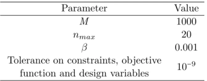
, the correspondent member is not shown. Finally, the parameters used in the optimization algorithm are presented in Table 1.
Table 1 Parameters used in the optimization algorithm.
Parameter Value
M 1000
nmax 20
β 0.001
Tolerance on constraints, objective
function and design variables 10
−9
4.1 Example 1
Figure 2 presents a ground structure that is subjected to the loading F = 10 kN. The ground
structure has the dimensions Lx = 2000 mm and Ly = 1000 mm. The initial cross-section
areas for the first local search are taken as 250 mm2
.
Figure 2 Ground structure of the Example 1.
note that the structures from Fig. 3(b) and Fig. 3(c) are slightly different, but have the same volume. It is important to remark that when the restart procedure was not used, the optimal structure found by the optimization algorithm was that presented in Fig. 3(c). It should be pointed out that other local optima were also found for this example that are not presented here. However, they are similar to the ones presented in Fig. 3(b) and Fig. 3(c).
V =3.1395×10⁵
mm3
Amax=80.8572 mm 2
(a)
V =3.2020×10⁵
mm3
Amax=60.9112 mm 2
(b)
V =3.2020×10⁵
mm3
Amax=64.2791 mm 2
(c)
Figure 3 Local optima found and their correspondent volumesV and maximum cross-section areaAmaxwhen
allowing the nodes to be moved by 500 mm from its original positions (Example 1).
Now, the same nodes are allowed to be moved up and down to position as far as 999 mm. The results are presented in Fig. 4, from where it can be seen that at least two local minima exist for this problem. Note that the volume of material used in each one is different, and these are indeed local optima. However, it seems that the structure from Fig. 4(a) is also the global optimum of this problem, since no better solution was found by the algorithm.
Taking a closer look at Fig. 3(a) one could conclude that this structure is the best solution available even when allowing the nodes to be moved farther than 500 mm, since the node that has been moved the most (the one from the right) is not linked to any bar. However, this is not true, as can be seen from the results from Fig. 4.
Finally, the same example is addressed again, but now only the cross-section areas are taken as design variables. Besides, this problem is solved twice: first assuming no upper bound for the cross-section areas and then assuming this upper bound to be equal to 60 mm2
. A solution with no upper bounds is presented in Fig. 5(a). Figures 5(b) and 5(c) show solutions when the upper bounds are taken into account.
When no upper bounds are defined, we have a simple sizing optimization problem that is a LP problem. Consequently, the solution found is a global optimum. The biggest cross-section area in this case is equal to 79.9312 mm2
V =3.1166×10⁵
mm3
Amax=73.0950 mm 2
(a)
V =3.1389×10⁵
mm3
Amax=74.3581 mm 2
(b)
Figure 4 Local optima found and their correspondent volumes V and maximum cross-section areaAmax
when allowing the nodes to be moved by 999 mm from its original positions (Example 1).
V =3.2036×105 mm3 Amax=79.9312 mm
2
(a)
V =3.6414×105mm3 Amax=60 mm
2
(b)
V =3.7754×105 mm3 Amax=60 mm
2
(c)
Figure 5 Optimum solution without upper bound for the cross-section areas (a), and some local optima found when the upper bound in cross-section areas is taken as 60mm2
(b) (c).
However, taking an upper bound equal to 60 mm2
enforces the algorithm to find alternatives to the solution presented in Fig. 5(a), since some cross-section areas in this case are bigger than 60 mm2
. Some solutions for this case are presented in Fig. 5(b) and Fig. 5(c). Note that the structure from Fig. 5(b) is symmetric about an horizontal axis, while the structure from Fig. 5(c) is not. This puts in evidence that when upper bounds for the cross-section areas are considered, local optima with different volume of material may exist. In fact, for some starting points the local search was unable to find a feasible solution. It should be mentioned that several local optima were found for this problem and not all of them are presented in Fig. 5.
4.2 Example 2
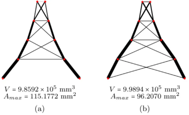
Figure 6 presents a ground structure that is subjected to three loading conditions. The ground structure has a total height of 4000 mm and a total width of 4000 mm. All nodes (except the nodes of the supports) are allowed to be moved left and right by the optimization algorithm, to positions as far as 1800 mm from its original position. The vertical and horizontal force values areF1= 10 kN andF2= 5 kN, respectively. Finally, symmetry of the structure about
Figure 6 Ground structure of the Example 2, subjected to three loading conditions.
V =9.8592×105mm3 Amax=115.1772 mm
2
(a)
V =9.9894×105mm3 Amax=96.2070 mm
2
(b)
Figure 7 Local optima for Example 2 and their correspondent volumes V and maximum cross-section area
Amax.
4.3 Example 3
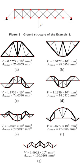
The third example is that presented in Fig. 8. The ground structure has a total height of 1000 mm and a total width of 8000 mm. All nodes of the upper chord are allowed to be moved up and down to positions as far as 10000 mm from its original position. The applied force isF =
10 kN. The initial values of the cross-section areas for the first local search are taken as 250 mm2
. Symmetry of the structure according to the vertical axis is enforced in this example. The results are presented in Fig. 9, and it can be seen that this problem have several local optima. It seems that the structure from Fig. 9(a) and Fig. 9(b) are the two global optima for this case. These two solutions are essentially the same, since the allowable stresses in tension and compression are the same. The same is true for the solutions from Fig. 9(c) and Fig. 9(d). It is important to note that the optimum solution found when no restart procedure was employed was that of Fig. 9(g), that is actually, among the solutions found, the worst one. This puts in evidence the importance of using global optimization strategies.
4.4 Example 4
Figure 8 Ground structure of the Example 3.
V =0.5772×106mm3 Amax=25.6859 mm
2
(a)
V =0.5772×106mm3 Amax=25.6859 mm
2
(b)
V =1.1939×106mm3 Amax=74.0320 mm
2
(c)
V =1.1939×106mm3 Amax=74.0320 mm
2
(d)
V =1.4026×106mm3 Amax=79.9947 mm
2
(e)
V =0.8777×106mm3 Amax=47.6602 mm
2
(f)
V =1.9992×106mm3 Amax=160.0268 mm
2
(g)
Figure 9 Local optima for Example 3 and their correspondent volumesV and maximum cross-section areaAmax.
The analytical solution for this problem is presented by Hemp [11], and it is a Michell’s structure as shown in Fig. 11. The minimum volume of the structure can also be obtained according to expressions presented by Hemp [11]. For this case, the expression that gives the minimum volume of material is
Vmin=(
F l σcσt)(
σc+σt) (1+
π
2), (10)
defined in Fig. 11 and 2F = 10kN.
Figure 10 Ground structure of the Example 4.
Figure 11 Optimal (Michell) truss solution according to Hemp [11].
Applying Eq. (10) to the example being studied, the minimum volume is 0.4113×106mm3.
It is important to remember that Michell’s structures are theoretical continuum solutions in the sense that they are, in general, composed of an infinite number of bars [11].
The solutions obtained by the optimization algorithm described here are the ones presented in Fig. 12. Again, a wide variety of local optima was obtained. Besides, the solution obtained by a single local search was the one from Fig. 12(a), that is clearly not the global optimum of the problem.
The global optima are the solutions presented in Fig. 12(e) and Fig. 12(f). Note that these two solutions are essentially the same, since we have assumed the same allowable stress in tension and compression. Besides, the volume of these two structures is 0.4191× 106 mm3,
which is very close to the theoretical value of 0.4113×106 mm3. The difference between these
two values can be explained by three reasons. First, Michell’s structures are composed of an infinite number of bars and this fact cannot be reproduced numerically. Second, the nodes of the ground structure from Fig. 10 are allowed to be moved only up and down, while the nodes of Michell’s structures can be placed everywhere. Third, the numerical solutions need to respect lower bounds for cross sectional areas, thus avoiding bars to disappear completely.
V =1.3536×106mm3 Amax=160.0001 mm
2
(a)
V =1.7150×106mm3 Amax=160.0001 mm
2
(b)
V =1.6663×106mm3 Amax=160.0002 mm
2
(c)
V =0.8744×106mm3 Amax=54.6255 mm
2
(d)
V =0.4191×106mm3 Amax=30.7535 mm
2
(e)
V =0.4191×106mm3 Amax=30.7535 mm
2
(f)
Figure 12 Local optima for Example 4 and their correspondent volumes V and maximum cross-section area
5 CONCLUSIONS
This paper presented an approach for the global optimization of truss structures that is based on a probabilistic restart procedure coupled with a local search algorithm. The resulting algorithm is able to guarantee local optimality and to asymptotically converge to the global optimum. Besides, the restart procedure is based on information from the previous iterations, and is not a purely random one, which may reduce computer time in the global optimization process.
The main advantage of the procedure proposed here is that the local search can be per-formed by efficient gradient based algorithms, thus ensuring that the solutions found by the algorithm are residual free. Finally, several loading conditions can be considered by including new sets of constraints.
At the end of the optimization procedure, the approach proposed here presents a set of local optima that are, in general, different from one another. In some cases, the designer may find some local optima more appealing than others (for some reasons apart from the material volume used) and thus choose some local optima instead of the global one.
The examples presented demonstrated that even for simple cases local minima, which are not global minima, may exist. Some of these local minima may even appear to be global optima at first glance. Besides, some problems may present several local optima, and in many cases the optimum solution found by a single local search is not the global one. This highlights the importance of considering global optimization procedures for the problem being addressed, since they can lead to much improved solutions. Finally, the last example demonstrated that the global optimization strategy proposed here was able to obtain the global optimum of the problem, by comparing the numerical solutions obtained with an analytical solution given in the literature.
References
[1] W. Achtziger. Topology optimization of discrete structures: in introduction in view of computational and nonsmooth aspects. In G.I.N. Rozvany, editor,Topology optimization in structural mechanics, Wien, 1997. Springer-Verlag.
[2] W. Achtziger. Simultaneous optimization of truss topology and geometry, revisited. In M. Bendsøoe, N. Olhoff, and O. Sigmund, editors,IUTAM Symposium on topological design optimization of structures, machines and materials: status and perspectives, pages 413–423, Berlin Heidelberg, New York, 2006. Springer.
[3] W. Achtziger. On simultaneous optimization of truss geometry and topology. Structural and Multidisciplinary Optimization, 33:285–305, 2007.
[4] W. Achtziger and M. Stolpe. Truss topology optimization with discrete design variables – guaranteed global optimality and benchmark examples. Structural and Multidisciplinary Optimization, 34:1–20, 2007.
[5] J. S. Arora. Introduction to optimum design. Elsevier, San Diego, 2004.
[6] K. J. Bathe. Finite element procedures. Prentice Hall, Englewood-Cliffs, 1996.
[7] G. D. Cheng and X. Guo. ε-relaxed approach in structural topology optimization.Structural Optimization, 13:258– 266, 1997.
[8] A. Dominguez, I. Stiharu, and R. Sedaghati. Practical design optimization of truss structures using the genetic algorithms. Research in Engineering Design, 17:73–84, 2006.
[10] R. T. Haftka and Z. G¨urdal. Elements of structural optimization. Kluwer, Dordrecht, 1992.
[11] W. S. Hemp. Optimum structures. Clarendon, Oxford, 1973.
[12] M. Kocvara and J. Zowe. How mathematics can help in design of mechanical structures. In D.F. Griffiths and Watson G.A., editors,Numerical Analysis, pages 76–93, Harlow, 1996. Longman.
[13] M. A. Luersen and R. Le Riche. Globalized Nelder-Mead method for engineering optimization. Computers & Structures, 82:2251–2260, 2004.
[14] G. C. Luh and C. Y. Lin. Optimal design of truss structures using ant algorithm. Structural and Multidisciplinary Optimization, 36:365–379, 2008.
[15] J. Nocedal and S. J. Wright.Numerical optimization. Springer-Verlag, Berlin, 1999.
[16] P. Pedersen. On the minimum mass layout of trusses. InSymposium on structural optimization, AGARD Conference Proceedings, volume 36, pages 189–192, 1970.
[17] P. Pedersen. Topology optimization of three-dimensional trusses. In M.P. Bendsøoe and C.A. Mota Soares, editors, Topology design of structures, pages 19–30, Dordrecht, 1993. Kluwer.
[18] H. Rahami, A. Kaveh, and Y. Gholipour. Sizing, geometry and topology of trusses via force method and genetic algorithm. Engineering Structures, 30:2360–2369, 2009.
[19] T. G. Ritto, R. H. Lopez, R. Sampaio, and J. E. Souza de Cursi. Robust optimization of a flexible rotor-bearing system using the Campbell diagram. Engineering Optimization, 43:77–96, 2011.
[20] G. I. N. Rozvany. Aims, scope, basic concepts and methods of topology optimization. In G.I.N. Rozvany, editor, Topology optimization in structural mechanics, Wien, 1997. Springer-Verlag.
[21] J. F. Schutte and A. A. Groenwold. Sizing design of truss structures using particle swarms.Structural and Multidis-ciplinary Optimization, 25:261–269, 2003.
[22] F. J. Solis and R. J. B. Wets. Minimization by random search techniques. Mathematics of Operations Research, 6:19–30, 1981.
[23] M. Stolpe and K. Svanberg. On the trajectories of the epsilon-relaxation approach for stress-constrained truss topology optimization.Structural and Multidisciplinary Optimization, 21:140–151, 2001.
[24] A. J. Torii and F. Biondini. A simple geometry optimization method for statically indeterminate trusses. In8th World Congress on Structural and Multidisciplinary Optimization, Lisbon, 2009.


![Figure 11 Optimal (Michell) truss solution according to Hemp [11].](https://thumb-eu.123doks.com/thumbv2/123dok_br/18884452.423490/12.892.340.597.355.493/figure-optimal-michell-truss-solution-according-hemp.webp)

