veloped for elastic bending response analysis of passenger ships with large multi-deck superstructures. The extension is mainly performed to enable the available method in or-der to study elastic bending behaviour of ships fitted with superstructures of any sizes and locations. Finite element method (FEM) is applied for solving the equilibrium equa-tions. Both hull and superstructure of the ship are modelled using beam elements. The connection between beam ele-ments representing hull and superstructure is made using specially developed spring box elements. The accuracy of the extended method is demonstrated using an available ex-perimental result. Then, two simplified structures, one rep-resenting a ship with a short superstructure and the other one representing a ship with a long superstructure, are anal-ysed in order to validate the extended coupled beam method against the finite element method. In spite of some existing simplifications in the extended formulation, it is very effec-tive in the early stages of ship structural design owing to its advantageous capability of rapid estimation of the longitudi-nal stress distributions along the height of ships at different stations.
Keywords
hull, superstructure, interaction, bending, Coupled Beam Method (CBM), Finite Element Method (FEM)
bFaculty of Marine Technology, Amirkabir Uni-versity of Technology, Tehran 15914 – Iran
Received 13 Dec 2010; In revised form 06 Apr 2011
∗Author email: [email protected]
1 INTRODUCTION
NOTATION
Ai cross-sectional area of the i-th beam
Aij nodal cross-sectional area of the i-th beam
Cij bending moment lever on the i-th beam due to the shearing force between the i-th
and j-th beams
dik distance between the upper fibre of the beam to the reference line
eij distance between the lower fibre of the beam to the reference line
E Modulus of elasticity
F external nodal forces matrix
Hij height of shear element between i-th andj-th beams
Ii sectional moment of inertia of thei-th beam
Iji nodal sectional moment of inertia of thei-th beam
K global stiffness matrix of system
Ki stiffness matrix ofi-th beam
kij transverse stiffness between the i-th and j-th beams
KShear stiffness matrix for the shearing springs
KT rans stiffness matrix for the transverse springs
Mi bending moment of thei-th beam
n number of beams
Ni axial force of the i-th beam
Nj(x) shape functions
pij transverse (vertical) distributed forces between the i-th and j-th beams
Qi shear force of the i-th beam
qi external force of thei-th beam
q∗
i approximate function for external force of the i-th beam
sij longitudinal distributed shear forces between the i-th and j-th beams
s∗
ij approximate function for longitudinal distributed shear forces between the i-th
and j-th beams
Tij shear stiffness between the i-th andj-th beams
ui axial displacement of thei-th beam
u∗
i approximate solution to axial displacement for the i-th beam
uij thej-th node of thei-th beam axial displacement
viM transverse deflection of the i-th beam caused by bending
viM∗ approximate solution to transverse displacement for the i-th beam
vji thej-th node of thei-th beam transverse displacement
X matrix of the degrees of freedom for the i-th beam
Xi first sectional moment of area of the i-th beam
Xji nodal first sectional moment of area of the i-th beam
Xs nodal displacement vector of system
δijv the relative displacement between beam i and beam j
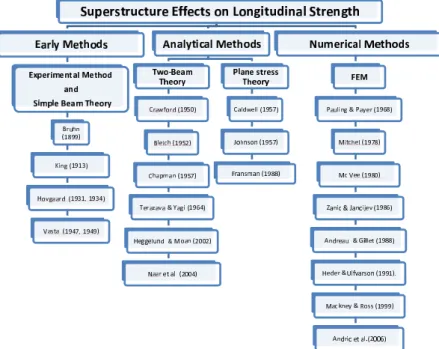
superstructure connection. He developed a theory of shear stresses in riveted and welded joints and applied it to discontinuities that occur in ship structures. Vasta [25, 26] seems to have been the first to use a measure of effectiveness to characterise the superstructure behaviour.
Figure 1 Overview of some of the key past studies on hull-superstructure interaction.
with the superstructure. Terazawa and Yagi [24] introduced the shear lag correction to the two-beam theory. The stresses were calculated using the energy approach and assuming pre-defined stress patterns for the structure. They also considered the effect of side openings on the structural behaviour. Simplified approach to generate global response of large catamarans with the large superstructure windows at the early stages of design using extended beam theory was presented by Heggelund and Moan [12]. Naar et al. [21] proposed a new approach called coupled beams method (CBM) to evaluate hull girder response of passenger ships. This method is based on the assumption that the global bending response of a modern passenger ship can be estimated by help of beams coupled to each other by distributed longitudinal and vertical springs.
Caldwell [5] presented a method based on plane stress theory in order to determine how the superstructure efficiency in hull bending strength varies with the ratio of its length to transverse dimensions, with the flexibility of the upper deck and with the distribution of bending moments applied on the ship. Johnson [16] also developed plane stress theory to study the stresses in deckhouses and superstructures. In his approach, the shear stress distribution along the edges of the deckhouse sides was assumed to be linear. The theory could take care of the possibility of deckhouse having several decks. Fransman [10] developed methods based on the plane stress theory and made an improvement with respect to Caldwell [5] approach.
tween beam elements representing hull and superstructure is made using specially developed spring box elements. The accuracy of the extended method is demonstrated using an available experimental result. Then, two simplified structures, one representing a ship with a short superstructure and the other one representing a ship with a long superstructure, are analysed in order to validate the extended coupled beam method against the finite element method. In spite of some existing simplifications in the extended formulation, it is very effective in the early stages of ship structural design owing to its advantageous capability of rapid estimation of the longitudinal stress distributions along the height of any ships at any specific stations.
2 COUPLED BEAM METHOD (CBM) 2.1 Brief description
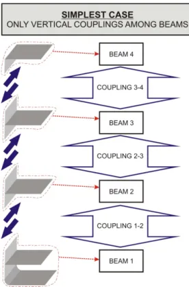
Naar et al. [21] proposed a coupled beam method (CBM) for longitudinal bending response analysis of passenger ships with long multi-deck superstructures above the deck. They con-sidered superstructures with the length equal to the ship’s length. In the approach presented by Naar et al., ship’s hull together with its long superstructure were modelled as a set of longitudinal beams, each having both bending stiffness and axial stiffness. Basic concept of discretisation of a multi-deck ship into a set of coupled beams is shown in Fig. 2. The beams are connected to each other using distributed springs.
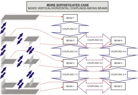
Figure 3 represents a simple case of discretisation in which only vertical couplings exist between beams. A more sophisticated case where both vertical and horizontal couplings exist between beams is shown in Fig. 4. Each beam in principle consists of an intersecting structure composed of horizontal and vertical substructures.
2.2 Governing equations [21]
A differential segment of the i-th beam with internal/external/coupling forces acting on it is shown in Fig. 5. The internal forces that are known from beam theory include axial force Ni,
shear force Qi and bending moment Mi. On the other hand, the coupling forces consist of
Figure 2 Basic concept of discretisation of a multi-deck ship into a set of coupled beams.
Figure 4 More sophisticated case of couplings among beams.
acting on the segment is qi that is resulted as a difference of the weight and buoyancy forces. Any of the loads that were defined above changes by a corresponding differential value towards the other section of thei-th beam segment as shown in Fig. 5.
Based on the formulation proposed by Naar et al., the reference line is fixed to the deck position and it may differ from the centroid position of the cross-section. dik and eij are respectively representing the distance between the upper and lower fibres of the beam to the reference line.
The equations of equilibrium for the forces acting on the i-th beam in both longitudinal and transverse directions are
∂Ni
∂x + n
∑
j=1
sij=0 (1)
∂Qi
∂x +
n
∑
j=1
pij =qi (2)
where the matrix of shear forcessij and also matrix of vertical forces pij are as follows
sij =⎧⎪⎪⎪⎨⎪⎪⎪ ⎩
sij 0
−sij
j>i j=i j<i
(3)
and
pij =⎧⎪⎪⎪⎨⎪⎪⎪ ⎩
pij 0
−pij
j>i j=i j<i
Figure 5 A differential segment of the i-th beam with internal/external/coupling forces acting on it.
The equilibrium equation for the moments about z-axis gives
∂2M
i
∂x2 +
n
∑
i=1
pij+∂(∑Cijsij)
∂x =qi (5)
where matrixC is
Cij=⎧⎪⎪⎪⎨⎪⎪⎪ ⎩
dij 0
−eij
j>i j=i j<i
(6)
Interaction between beams is defined using the coupling equations. The coupling equa-tions are to be written for both shear forces and vertical forces. Shear coupling between two neighbouring beams is shown schematically in Fig. 6. Due to the shear element with the shear stiffnessTij, displacement discontinuity δiju causes shear forces sij between beams. It is assumed that this shear force is constant over length dx. Thus, this force may be considered as the response of distributed horizontal spring between the two neighbouring beams. Shear stiffness depends on the effective heightHij of the shear element and also its effective area. In this case, as shown in Fig. 6, the effective height is equal to the deck spacing. Therefore, the approximate shear force in the side shell or in the longitudinal bulkhead is equal to
sij(x)=Tij(x)δiju(x) (7)
Figure 6 Shear element approach for definition of shear coupling between beams.
δiju =uj+eji ∂vjM
∂x −ui+dij ∂viM
∂x (8)
where viM is the deflection of beam i caused by bending. Substituting Eq. (8) into Eq. (7) results in the following equation for the shear force
sij =Tij⎛
⎝uj−Cji
∂vjM
∂x −ui+Cij ∂vM
i
∂x
⎞
⎠ (9)
And the longitudinal shear stiffness matrix is
Tij={
Tij 0
j≠i
j=i (10)
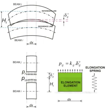
The next type of coupling is vertical coupling. This type of coupling is of great importance when the superstructure is weakly supported. This condition is well described by Bleich [3]. The interaction between beams i and j is described with distributed vertical springs in Fig. 7. Vertical coupling force pij depends on vertical coupling stiffness kij and relative deflection
δijv, which is the difference between beam deflections viand vj. Hence
Pij(x)=kij(x)δvij(x)=kij(x) (vj(x)−vi(x)) (11)
Using the beam theory, the relations between the internal forces and displacements are defined assuming that the material follows Hooke’s law. If axial displacementui and deflection viM are known for beam i, then bending momentMi and axial forces Ni are, see Crisfield [8]
Mi=−EIi
∂2viM
∂x2 +EXi
∂ui
Ni=EAi∂ui
∂x −EXi ∂2vM
i
∂x2 (13)
where parametersEAiand EIiare the axial stiffness and the bending stiffness of beamiwith respect to the reference axis and EXi is the value which modifies the internal forces if the reference line differs from the centroid of the cross-section. Matrices EAi, EIi and EXi are diagonal.
Figure 7 Elongation element approach for definition of vertical coupling between beams.
2.3 Summary of equations to be solved
The following equations are to be solved in order to assess bending response of a ship using coupled beam method
⎧⎪⎪⎪⎪ ⎪⎪⎪ ⎨⎪⎪⎪ ⎪⎪⎪⎪ ⎩
∂Ni
∂x + ∑ n
j=1sij=0 ∂2Mi
∂x2 +∑ n
i=1pij+∂(∑C∂xijsij)=qi Mi=−E Ii∂
2 vMi
∂x2 +EXi ∂ui
∂x
Ni=EAi∂u∂xi +EXi∂ 2
viM
∂x2
(14)
Eliminating Mi and Ni in above equations, result in the following equations
−
n
∑
j=1
sij=
∂ ∂x(EAi
∂ui
∂x −EXi ∂2viM
With such an assumption, shape functions are defined along the ship’s hull and superstructure. In case of a ship having a short superstructure, the values of longitudinal shear force and vertical transverse force are not equal to zero at both ends of superstructure. Therefore, some modifications are necessary to be performed within the approach developed by Naar et al. in order to make it applicable to other types of ships having superstructures of any lengths. This is the main reason behind works presented in this manuscript.
3 EXTENDED FORMULATION 3.1 General
In order to resolve existing inabilities in the approach presented by Naar et al. regarding bending response analysis of ships with short superstructures, a new method is provided in this paper. The adopted concept for discretisation of ship structure into different beam and spring elements is shown schematically in the Fig. 8. As can be seen in Fig. 8, both hull and superstructure are modelled as beams consisting of a number of beam elements. In the connecting region between hull and superstructure, the nodes are so located to have the same abscissa. The beam elements are of three-node type, having a total number of six degrees of freedom, so that the variations in the axial force can be considered. The reference line is considered at the deck level.
The beams representing hull and superstructure are connected to each other using the so-called ‘spring box elements’. The stiffness matrix of these spring box elements is derived using equilibrium conditions. Any spring box elements consist of 9 transverse springs and also 9 shear springs, Fig. 9. The transverse springs and shear springs are simulating respectively vertical forces and shear forces acting between the two beam elements, one inside the hull and the other one inside the superstructure.
The governing equations to be solved were summarised in Section 2.3. The boundary conditions are of free-free type. The Galerkin method [15] is adopted in order to solve the set of equations. Using the Galerkin method, the finite element equations are formulated.
The length of the ship is divided into m intervals. The first node is chosen at the after
perpendicular position, while the last node is placed at the forward perpendicular. Each of the intervals includes three nodes. u∗
Figure 8 Adopted concept for discretisation of ship structure into different beam and spring elements.
Figure 9 Different components within any of spring box elements.
functions in i-th interval. These approximate solutions are considered as linear combination of the corresponding nodal deflections in the following manner
u∗ i =
9 ∑
j=7
xijNj(x) (17)
viM∗=
6 ∑
j=1
xijNj(x) (18)
Degrees of freedom in above equations are as follows
Xi=[ xi1 xi2 xi3 xi4 xi5 xi6 xi7 xi8 xi9 ]
⎨⎪⎪⎪ ⎪⎪⎪⎪⎪ ⎪⎪⎪⎪⎪ ⎪⎪⎪⎪⎪ ⎪⎪⎪⎩
N6[x]=−L + L2 − L3 + L4
N7[x]=1−3Lx+2x
2
L2
N8[x]= 4Lx−4x
2
L2
N9[x]=−Lx +2x
2
L2
The residuals would be
R1=
∂ ∂x(EAi
∂u∗ i
∂x −EXi ∂2vM∗
i
∂x2 )+
n
∑
j=1
s∗
ij (20)
R2=
∂2
∂x2(−EIi
∂2vM∗ i
∂x2 +EXi
∂u∗ i
∂x )+
∂(∑Cijs∗ij)
∂x +
n
∑
i=1
p∗
ij−q∗i (21)
Based on the Galerkin method, in order to have minimum error, the functionsu∗
i and vM∗i have to satisfy the following equations
∫x1x2Nm(x)⎛ ⎝
∂ ∂x(EAi
∂u∗ i
∂x −EXi ∂2vM∗i
∂x2 )+
n
∑
j=1
s∗ ij
⎞
⎠dx=0 m=7,8,9 (22)
∫x1x2Nm(x)⎛ ⎝
∂2
∂x2(−E Ii
∂2vM∗i
∂x2 +EXi
∂u∗ i
∂x )+
∂(∑Cijs∗ij)
∂x +
n
∑
i=1
p∗ ij−qi∗
⎞
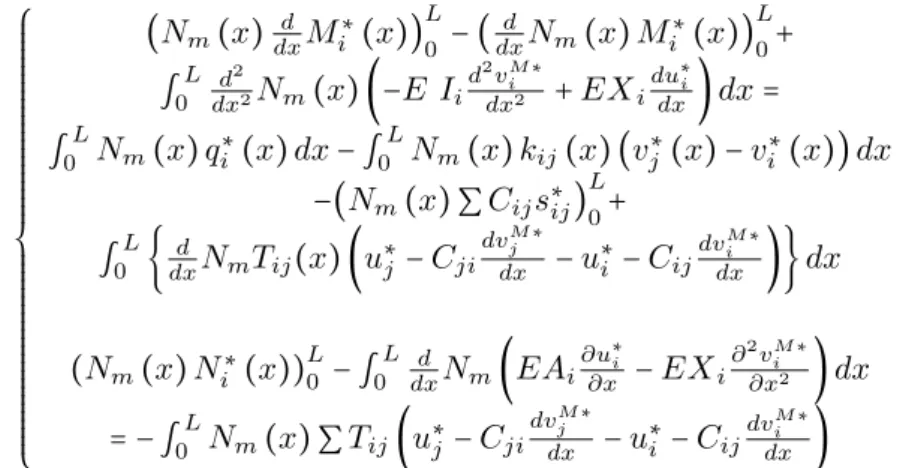
⎧⎪⎪⎪⎪ ⎪⎪⎪⎪⎪ ⎪⎪⎪⎪⎪ ⎪⎪⎪⎪⎪ ⎪⎪⎪⎪⎪ ⎨⎪⎪⎪ ⎪⎪⎪⎪⎪ ⎪⎪⎪⎪⎪ ⎪⎪⎪⎪⎪ ⎪⎪⎪⎪⎪ ⎪⎩
(Nm(x)dxd Mi∗(x)) L
0 −(
d
dxNm(x)M ∗ i (x))
L
0+ ∫0L
d2
dx2Nm(x) (−E Ii d2vM∗
i
dx2 +EXi du∗
i
dx)dx=
∫0LNm(x)q∗i (x)dx−∫ L
0 Nm(x)kij(x) (vj∗(x)−vi∗(x))dx
−(Nm(x)∑Cijs∗ij) L
0+ ∫0L{
d
dxNmTij(x) (u∗j −Cji dvM∗
j
dx −u∗i −Cijdv
M∗
i
dx )}dx
(Nm(x)Ni∗(x)) L
0 −∫
L
0
d
dxNm(EAi ∂u∗
i
∂x −EXi ∂2
vM∗
i
∂x2 )dx
=−∫L
0 Nm(x)∑Tij(u∗j −Cji dvM∗
j
dx −u∗i −Cijdv
M∗
i
dx )
(24)
The stiffness matrices for the beam elements and spring box elements can be easily obtained using Eq. (24). More details on these are given in the next sections.
3.2 Assembling algorithm
After derivation of stiffness matrices for hull beam elements, superstructure beam elements and also spring box elements, the global stiffness matrix of the whole ship structure is assembled. Since the shear force and bending moment are zero at both ends of the ship, in order to solve the finite element equations, singular points should be eliminated so that rigid body motion of the ship is prevented. The resulting set of finite element equations is then solved. Figure 10 shows the flow of steps from beginning towards the solution.
Since the sectional properties of a ship are generally variable along its length, it would be more accurate if the sectional properties of the beam elements can also vary along their length. Therefore, the quantitiesEAi,EXi and EIi are defined in the new formulation as follows
⎧⎪⎪⎪ ⎨⎪⎪⎪ ⎩
EIi[x]=EI1i ∗N7[x]+EIi2∗N8[x]+EIi3∗N9[x]
EXi[x]=EX1i ∗N7[x]+EXi2∗N8[x]+EXi3∗N9[x]
EAi[x]=EA1i ∗N7[x]+EAi2∗N8[x]+EAi3∗N9[x]
(26)
where Ii, Ai and Xi are second moment of inertia, cross-sectional area and first sectional
moment of area at node number i of the beam element, which can be calculated by the
following equations
EIi= ∑
over the cross−section
EjAjZj2
EXi= ∑
over the cross−section
EjAjZj
EAi= ∑
over the cross−section
EjAj
Using above definitions, the stiffness matrix takes the following form
Ki=KEA1.EAi1+KEA2.EAi2+KEA3.EA3i +KEX1.EXi1+KEX2.EXi2+KEX3.EXi3+
+KEI1.EIi1+KEI2.EIi2+KEI3.EIi3
(27)
The vector of degrees of freedom for i-th beam element is[vi
1 v2i vi3 θi1 θ2i θ3i ui1 ui2 ui3]
T
3.4 Stiffness matrix of the spring box elements
Spring box elements are used in order to simulate the connection between beam elements of the hull and beam elements of the superstructure. The forces acting on the beam elements from the spring box elements are ∑nj=1sij, ∑nj=1pij and ∑nj=1Cijsij, which are respectively representing axial force per unit length, transverse force per unit length and bending moment per unit length.
Any one of spring box elements has 6 nodes, a total of 18 degrees of freedom, shear stiffness and transverse vertical stiffness. The shear stiffness matrix and transverse vertical matrix are
KShear= ⎡⎢ ⎢⎢ ⎢⎢ ⎢⎢ ⎣ −C 2
ijTijA CijTijB CijCjiTijA −CijTijB CijTijB −TijD −CjiTijB TijD CijCjiTijA −CjiTijB −C2
jiTijA CjiTijB
−CijTijB TijD CjiTijB −TijD
⎤⎥ ⎥⎥ ⎥⎥ ⎥⎥ ⎦ = ⎡⎢ ⎢⎢ ⎢⎢ ⎢⎢ ⎢⎢ ⎢⎢ ⎢⎣
1≤k≤6 7≤k≤9 1≤k≤6 7≤k≤9
1≤m≤6 [−∫L
0 C 2 ijTijN
′ mN
′
kdx] [∫ L 0 CijTijN
′
mNkdx] [∫0LCijCjiTijN ′ mN
′
kdx] [−∫
L 0 CijTijN
′ mNkdx] 7≤m≤9 [∫0LCijTijNm′ Nkdx] [−∫0LTijNmNkdx] [−∫
L 0 CjiTijN
′
mNkdx] [∫0LTijNmNkdx] 1≤m≤6 [∫L
0 CijCjiTijN ′ mN
′
kdx] [−∫
L 0 CjiTijN
′
mNkdx] [−∫
L 0 C
2 jiTijN
′ mN
′
kdx] [∫ L 0 CjiTijN
′ mNkdx] 7≤m≤9 [−∫L
0 CijTijN ′
mNkdx] [∫0LTijNmNkdx] [∫0LCjiTijN ′
mNkdx] [−∫0LTijNmNkdx]
⎤⎥ ⎥⎥ ⎥⎥ ⎥⎥ ⎥⎥ ⎥⎥ ⎥⎦ (28) and
KT rans = ⎡⎢ ⎢⎢ ⎢⎢ ⎢⎢ ⎢⎢ ⎣
[−∫0LkijNkNmdx] 0 [∫
L
0 kijNkNmdx] 0
0 0 0 0
[∫L
0 kijNkNmdx] 0 [−∫
L
0 kijNkNmdx] 0
0 0 0 0
⎤⎥ ⎥⎥ ⎥⎥ ⎥⎥ ⎥⎥ ⎦ = ⎡⎢ ⎢⎢ ⎢⎢ ⎢⎢ ⎣
−kijE 0 kijE 0
0 0 0 0
kijE 0 −kijE 0
0 0 0 0
⎤⎥ ⎥⎥ ⎥⎥ ⎥⎥ ⎦ (29)
Matrices A,B,D and E are given in the appendix.
3.5 Elimination of singular points of solution of finite element equations
The global stiffness matrix of the whole ship is singular, because there are not enough support constraints to prevent its rigid body motion. In these cases, Singular Value Decomposition (SVD) offers a better solution in many respects. All matrices have a unique decomposition as multiplication of three matrices, a square orthogonal matrix, a diagonal matrix and a square
orthogonal matrix. Therefore, K, the global stiffness matrix of system, can be written as
bellow
K=U.diag.VT (30)
where U and V are square real and orthogonal. diag is a diagonal matrix that contains the
singular values. In terms of U,V, and diag, the system is readily solved
tively.
3.6 Implementation
Newly extended formulation was implemented in a code that was written in MATLAB envi-ronment. The code creates the set of finite element equations for the whole ship structure considering the couplings among beam elements of the hull and superstructure. The inputs of the code are typically coordinates of the nodes, beam element connectivity matrix, spring connectivity matrix and also vector of the loads. The outputs of the code consist of deflection components at the nodes, internal forces and moments at the nodes and also longitudinal stress at the nodes.
4 VALIDATION
Mackney and Rose [18] tested a simple ship model with the scale of 1/60 in a four-point bending mechanism. The model had a length of 2m, a breadth of 0.25m, a hull height of 0.167m and a superstructure height of 0.117m. The experimentally obtained deflections for the model are shown in Fig. 11 with the marked points. The numerical results using the developed code are also shown in the Fig. 11 with the solid line. As can be seen, a very good correlation exists among the results.
5 NUMERICAL EXPERIMENTS AND DISCUSSIONS
Two models are created numerically and their bending responses are assessed using the de-veloped code. In order to examine validity of the results obtained based on the extended formulation; the same models are analysed using ANSYS finite element code [23]. Different paths are considered along the models where longitudinal stress distributions obtained based on the present formulation and ANSYS are compared with each at them. All the forces ap-plied on the models are self-balanced. That means there are no forces acting on the imaginary support considered for the model. This support could be placed at any location on the natural axis of the section. Herein, in order to prevent rigid body motion of the models, a point on the midlength of the hull, but located on the neutral axis of the section, is restrained against mo-tion. Elements of SHELL63 [23] type were used in order to discretise the models. SHELL63 element has both bending and membrane capabilities. Both in-plane and normal loads are permitted. The element has six degrees of freedom at each node: translations in the nodal x, y, and z directions and rotations about the nodal x, y, and z axes. Stress stiffening and large deflection capabilities are included.
5.1 Case study 1: box girder model with a superstructure shorter than the hull
Model number 1 is a box girder model in which the superstructure has a length smaller than that of the hull. Geometrical specifications of the model are shown in Fig. 12(a). Loading distribution for the model is also given in Fig. 12(b). In order to investigate longitudinal stress distributions for the model, 6 equidistant paths are considered between both ends of the superstructure (Fig. 12(a)).
(a) Geometrical specifications
(b) Load diagram
side openings may be compensated using simple empirical equations that can be implemented in the present extended formulation. This remains as a future work.
Figure 14, 15, 16 and 17 also demonstrate this fact that the superstructure is contributing to the bending strength of the ship’s hull. Again good correlations are observed among the results of the developed code and ANSYS.
Figure 13 Comparison of longitudinal stresses along height of ship at the location of path 1 in model no. 1.
Figure 15 Comparison of longitudinal stresses along height of ship at the location of path 3 in model no. 1.
Figure 16 Comparison of longitudinal stresses along height of ship at the location of path 4 in model no. 1.
Figure 17 Comparison of longitudinal stresses along height of ship at the location of path 5 in model no. 1.
Figure 19 Geometrical specifications for the model no. 2.
Figure 20 Comparison of longitudinal stresses along height of ship at the location of path 2 in model no. 2.
6 CONCLUSIONS
This paper was aimed at investigation bending response of the ships considering the contribu-tion of the superstructure. The coupled beam method developed by Naar et al. was further extended in a way that the resulting formulation could be capable of analysing the elastic bending response of the ships having superstructures of any lengths. The new extended for-mulation was coded in MATLAB environment and then it was validated against some available experimental data. Furthermore, some new cases were generated and their behaviours were examined using the extended formulation and ANSYS software. The results of the extended formulation for the numerical models were then compared with those results obtained using the finite element method and relatively good correlations were observed among them.
The extended formulation of the coupled beam method is so much effective in terms of CPU time and accuracy that can be easily implemented in the algorithms for assessment of the longitudinal bending strength of ship structures, considering the contribution coming from superstructures.
Improvements of the extended formulation in order to enable it to assess the stresses at discontinuities more accurately, such as hull-superstructure connections and side openings, are recommended to be performed as future works.
References
[1] C. Andreau and L. Gillet. Structural design improvements of passenger ships. In IMAS 88, The Design and
Development of Passenger Ships, 1988.
[2] J. Andric, V. Zanic, and M. Grgic. Superstructure deck effectiveness in longitudinal strength of livestock carrier. In
The 17th Symposium on Theory and Practice of Shipbuilding, SORTA 2006, Rijeka, Croatia, 2006.
[3] H.H. Bleich. Non-linear distribution of bending stresses due to distortion of cross-section. J Appl Mech, 29:95–104, 1952.
[4] J. Bruhn. The stress at the discontinuities in a ship’s structure. Trans RINA, pages 57–63, 1899.
[5] J.B. Caldwell. The effect of superstructure on the longitudinal strength of ships. Trans RINA, 99(4):664–681, 1957.
[6] J.C. Chapman. The interaction between a ship’s hull and long superstructure. Trans RINA, 99(4):618–633, 1957.
[7] L. Crawford. Theory of long ship’s superstructure. Trans SNAME, 58:693–732, 1950.
[8] M.A. Crisfield. Non-linear finite element analysis of solids and structures, volume 1. John Willey & Sons, West Sussex, England, 1991.
[9] J.G. de Oliveira. Hull-deck interaction. In J.H. Evands, editor,Ship structural design concepts, second cycle, pages 160–278, USA, 1983. Cornell Maritime Press.
[10] J. Fransman. The influence of passenger ship superstructures on the response of the hull girder. Trans RINA, 131:57–71, 1988.
[11] M. Heder and A. Ulfvarson. Hull beam behavior of passenger ships. Marine structure, 4:17–34, 1991.
[12] S.E. Heggelund and T. Moan. Analysis of global loads effects in catamarans.Journal of Ship Research, 46(2):81–91, 2002.
[13] W. Hovgaard. A new theory of the distribution of shearing stresses in riveted and welded connection and its application to discontinuities in the structure of a ship. Trans RINA, pages 52–59, 1931.
1968.
[23] Swanson Analysis Systems Inc., Houston. ANSYS User’s Manual (Version 7.1), 2003.
[24] K. Terazava and J. Yagi. Stress distribution in deckhouse and superstructure. The Society of Naval Architects of
Japan, 60th Anniversary Series, 9:51–150, 1964.
[25] J. Vasta. Structural tests on the libery ship S.S. Philip Schuyer. Trans SNAME, 55:391–396, 1947.
[26] J. Vasta. Structural tests on the passenger ship S.S. President Wilson – Interaction between superstructure and main hull girder. Trans SNAME, 57:253–306, 1949.
APPENDIX
KEA1=
⎡⎢ ⎢⎢ ⎢⎢ ⎢⎢ ⎢⎢ ⎢⎢ ⎢⎢ ⎢⎢ ⎢⎢ ⎢⎢ ⎣
0 0 0 0 0 0 0 0 0
0 0 0 0 0 0 0 0 0
0 0 0 0 0 0 0 0 0
0 0 0 0 0 0 0 0 0
0 0 0 0 0 0 0 0 0
0 0 0 0 0 0 0 0 0
0 0 0 0 0 0 37
30L − 22 15L
7 30L
0 0 0 0 0 0 −15L22
8 5L −
2 15L
0 0 0 0 0 0 7
30L − 2 15L − 1 10L ⎤⎥ ⎥⎥ ⎥⎥ ⎥⎥ ⎥⎥ ⎥⎥ ⎥⎥ ⎥⎥ ⎥⎥ ⎥⎥ ⎦
KEA2=
⎡⎢ ⎢⎢ ⎢⎢ ⎢⎢ ⎢⎢ ⎢⎢ ⎢⎢ ⎢⎢ ⎢⎢ ⎢⎢ ⎣
0 0 0 0 0 0 0 0 0
0 0 0 0 0 0 0 0 0
0 0 0 0 0 0 0 0 0
0 0 0 0 0 0 0 0 0
0 0 0 0 0 0 0 0 0
0 0 0 0 0 0 0 0 0
0 0 0 0 0 0 6
5L − 16 15L −
2 15L
0 0 0 0 0 0 −15L16
32 15L −
16 15L
0 0 0 0 0 0 −15L2 −
16 15L 6 5L ⎤⎥ ⎥⎥ ⎥⎥ ⎥⎥ ⎥⎥ ⎥⎥ ⎥⎥ ⎥⎥ ⎥⎥ ⎥⎥ ⎦
KEA3=
⎡⎢ ⎢⎢ ⎢⎢ ⎢⎢ ⎢⎢ ⎢⎢ ⎢⎢ ⎢⎢ ⎢⎢ ⎢⎢ ⎣
0 0 0 0 0 0 0 0 0
0 0 0 0 0 0 0 0 0
0 0 0 0 0 0 0 0 0
0 0 0 0 0 0 0 0 0
0 0 0 0 0 0 0 0 0
0 0 0 0 0 0 0 0 0
0 0 0 0 0 0 −10L1 −
2 15L
7 30L
0 0 0 0 0 0 −15L2
8 5L −
22 15L
0 0 0 0 0 0 30L7 −15L22
37 30L ⎤⎥ ⎥⎥ ⎥⎥ ⎥⎥ ⎥⎥ ⎥⎥ ⎥⎥ ⎥⎥ ⎥⎥ ⎥⎥ ⎦
KEX1=
⎡⎢ ⎢⎢ ⎢⎢ ⎢⎢ ⎢⎢ ⎢⎢ ⎢⎢ ⎢⎢ ⎢⎢ ⎢⎢ ⎣
0 0 0 0 0 0 237
35L2 −
988 105L2
277 105L2
0 0 0 0 0 0 −5L322
128 15L2 −
32 15L2
0 0 0 0 0 0 −35L132
92 105L2 −
53 105L2
0 0 0 0 0 0 92
35L − 356 105L
16 21L
0 0 0 0 0 0 32
35L −
64 35L
32 35L
0 0 0 0 0 0 1
35L 8 105L − 11 105L 237
35L2 −
32 5L2 −
13 35L2 92 35L 32 35L 1
35L 0 0 0
−105L9882
128 15L2
92 105L2 −
356 105L −
64 35L
8
105L 0 0 0
277 105L2 −
32 15L2 −
53 105L2 16 21L 32 35L − 11
105L 0 0 0
KEX3= ⎡⎢ ⎢⎢ ⎢⎢ ⎢⎢ ⎢⎢ ⎢⎢ ⎢⎢ ⎢⎢ ⎢⎢ ⎢⎢ ⎣
0 0 0 0 0 0 105L532 −
92 105L2
13 35L2
0 0 0 0 0 0 15L322 −
128 15L2
32 5L2
0 0 0 0 0 0 −105L2772
988 105L2 −
237 35L2
0 0 0 0 0 0 −105L11
8 105L
1 35L
0 0 0 0 0 0 32
35L −
64 35L
32 35L
0 0 0 0 0 0 16
21L − 356 105L 92 35L 53 105L2 32 15L2 −
277 105L2 −
11 105L
32 35L
16
21L 0 0 0
−105L922 −
128 15L2 988 105L2 8 105L − 64 35L − 356
105L 0 0 0
13 35L2
32 5L2 −
237 35L2 1 35L 32 35L 92
35L 0 0 0
⎤⎥ ⎥⎥ ⎥⎥ ⎥⎥ ⎥⎥ ⎥⎥ ⎥⎥ ⎥⎥ ⎥⎥ ⎥⎥ ⎦
KEI1= ⎡⎢ ⎢⎢ ⎢⎢ ⎢⎢ ⎢⎢ ⎢⎢ ⎢⎢ ⎢⎢ ⎢⎢ ⎢⎢ ⎣
−105L96583
1088 15L3
2042 105L3 −
2638 105L2 −
416 15L2 −
20
7L2 0 0 0
1088 15L3 −
5632 105L3 −
1984 105L3 2176 105L2 768 35L2 64
21L2 0 0 0
2042 105L3 −
1984 105L3 −
58 105L3
22 5L2
608 105L2 −
4
21L2 0 0 0
−105L26382
2176 105L2
22 5L2 −
2419 315L −
2032 315L −
199
315L 0 0 0
−15L4162
768 35L2
608 105L2 −
2032 315L −
2944 315L −
304
315L 0 0 0
−7L202
64 21L2 −
4 21L2 −
199 315L −
304 315L
83
315L 0 0 0
0 0 0 0 0 0 0 0 0
0 0 0 0 0 0 0 0 0
0 0 0 0 0 0 0 0 0
⎤⎥ ⎥⎥ ⎥⎥ ⎥⎥ ⎥⎥ ⎥⎥ ⎥⎥ ⎥⎥ ⎥⎥ ⎥⎥ ⎦
KEI2=
⎡⎢ ⎢⎢ ⎢⎢ ⎢⎢ ⎢⎢ ⎢⎢ ⎢⎢ ⎢⎢ ⎢⎢ ⎢⎢ ⎣
−21L11123
1024 21L3
88 21L3 −
796 105L2 −
64 3L2
12
35L2 0 0 0
1024 21L3 −
2048 21L3
1024 21L3
832
105L2 0 −
832
105L2 0 0 0
88 21L3
1024 21L3 −
1112 21L3 −
12 35L2
64 3L2
796
105L2 0 0 0
−105L7962
832 105L2 −
12 35L2 −
652 315L −
544 315L
8
45L 0 0 0
−3L642 0
64 3L2 −
544 315L −
5632 315L −
544
315L 0 0 0
12 35L2 −
832 105L2 796 105L2 8 45L − 544 315L − 652
315L 0 0 0
0 0 0 0 0 0 0 0 0
0 0 0 0 0 0 0 0 0
0 0 0 0 0 0 0 0 0
KEI3= ⎡⎢ ⎢⎢ ⎢⎢ ⎢⎢ ⎢⎢ ⎢⎢ ⎢⎢ ⎢⎢ ⎢⎢ ⎢⎢ ⎣
−105L583 −
1984 105L3
2042 105L3
4 21L2 −
608 105L2 −
22
5L2 0 0 0
−105L19843 −
5632 105L3
1088 15L3 −
64 21L2 −
768 35L2 −
2176
105L2 0 0 0
2042 105L3
1088 15L3 −
9658 105L3 20 7L2 416 15L2 2638
105L2 0 0 0
4 21L2 −
64 21L2 20 7L2 83 315L − 304 315L − 199
315L 0 0 0
−105L6082 −
768 35L2
416 15L2 −
304 315L −
2944 315L −
2032
315L 0 0 0
−5L222 −
2176 105L2
2638 105L2 −
199 315L −
2032 315L −
2419
315L 0 0 0
0 0 0 0 0 0 0 0 0
0 0 0 0 0 0 0 0 0
0 0 0 0 0 0 0 0 0
⎤⎥ ⎥⎥ ⎥⎥ ⎥⎥ ⎥⎥ ⎥⎥ ⎥⎥ ⎥⎥ ⎥⎥ ⎥⎥ ⎦ A= ⎡⎢ ⎢⎢ ⎢⎢ ⎢⎢ ⎢⎢ ⎢⎢ ⎢⎣ 278 105L −
256 105L −
22 105L 13 210 8 21 − 1 70 −105256L
512 105L −
256 105L −
8 105 0
8 105 −10522L −
256 105L 278 105L 1 70 − 8 21 − 13 210 13 210 − 8 105 1 70 2L 45 − 4L 315 − L 126 8
21 0 −
8 21 − 4L 315 128L 315 − 4L 315 −701
8 105 − 13 210 − L 126 − 4L 315 2L 45 ⎤⎥ ⎥⎥ ⎥⎥ ⎥⎥ ⎥⎥ ⎥⎥ ⎥⎦ B= ⎡⎢ ⎢⎢ ⎢⎢ ⎢⎢ ⎢⎢ ⎢⎢ ⎢⎣
−101210 − 4 7
11 210 8
15 0 −
8 15 −21011
4 7 101 210 13L 420 − L 35 − L 420 −1058L
16L
105 − 8L
105 −420L −
L 35 13L 420 ⎤⎥ ⎥⎥ ⎥⎥ ⎥⎥ ⎥⎥ ⎥⎥ ⎥⎦ D= ⎡⎢ ⎢⎢ ⎢⎢ ⎣ 2L 15 L 15 − L 30 L 15 8L 15 L 15 −30L 15L 215L
⎤⎥ ⎥⎥ ⎥⎥ ⎦ E= ⎡⎢ ⎢⎢ ⎢⎢ ⎢⎢ ⎢⎢ ⎢⎢ ⎢⎢ ⎢⎣
−5233465L − 4L
63 − 131L
6930 − 19L2
2310
8L2
693
29L2
13860 −463L −
128L
315 − 4L
63 −
2L2
315 0
2L2
315 −1316930L −463L −5233465L −29L
2
13860 − 8L2
693
19L2
2310 −19L
2
2310 − 2L2
315 − 29L2
13860 − 2L3
3465
L3
1155
L3
4620 8L2
693 0 −
8L2
693
L3
1155 − 32L3
3465
L3
1155 29L2
13860
2L2
315
19L2
2310
L3
4620
L3
1155 − 2L3