MAXIMUM RESPIRATORY PRESSURE MEASURING SYSTEM:
CALIBRATION AND EVALUATION OF UNCERTAINTY
José L. Ferreira
∗ [email protected]Nadja C. Pereira
∗ [email protected]Marconi Oliveira Jr.
∗Flávio H. Vasconcelos
∗ [email protected]Verônica F. Parreira
†Carlos J. Tierra-Criollo
∗∗Department of Electrical Engineering
Federal University of Minas Gerais Belo Horizonte – Brazil
†Department of Physiotherapy
Federal University of Minas Gerais Belo Horizonte – Brazil
ABSTRACT
The objective of this paper is to present a methodology for the evaluation of uncertainties in the measurements results obtained during the calibration of a digital manovacuometer prototype (DM) with a load cell sensor pressure device incorporated. Calibration curves were obtained for both pressure sensors of the DM using linear regression by weighted least squares method (WLS). Two models were built to evaluate uncertainty. One takes into account the information listed in the sensor datasheet, resulting in the maximum permissible measurement error of the manovacuometer, and the other on the WLS implemented during calibration. Considering a range of ten calibration points, it was found that calibration procedure designed using WLS modeling indicates that the range of measurement uncertainty extends from 0.2 up to 0.5 kPa. This is inside the manufacter range that extends from 1.5 up 3.5 kPa, showing adequacy for use.
Artigo submetido em 26/08/2009 (Id.: 01030) Revisado em 24/03/2010, 26/10/2010
Aceito sob recomendação do Editor Associado Prof. Sebastian Yuri Cavalcanti Catunda
KEYWORDS: Calibration, measurement uncertainty, maximum respiratory pressures measuring system, weighted least squares.
RESUMO
Medidor de pressões respiratórias máximas: calibração e cálculo da incerteza
construído com base nas informações dodatasheetdo sensor, que varia entre 1,5 e 3,5 kPa, evidenciando que o protótipo está adequado para uso.
PALAVRAS-CHAVE: Calibração, incerteza de medição, medidor de pressões respiratórias máximas, mínimos quadrados ponderado.
1
INTRODUCTION
A number of the advances that have revolutionized medicine in recent years is being backed by sophisticated electronic instruments that can detect many type of phenomena or substances related to illness. In consequence, clinics and hospitals are acquiring devices that are being used in diagnostic as well in health care.
According to the Guide (GUM, 2003), the result of a measurement only will be complete if it is composed by the measured quantity value and the measured uncertainty, being important to the quality control of products and services. In this context, reliable measurement in health care applications is fundamental for a correct final diagnosis of diseases. A wrong evaluated value for the measurements can affect any decision about the health condition of a patient (Lira, 2002; Parvis and Vallan, 2002).
Aware of this fact, Brazilian Ministry of Health (MS) and the National Institute of Metrology, Standardization and Industrial Quality (INMETRO), the local NMI (National Measurement Institute), have established the compulsory tests for medical and hospital equipment (MHE) certification (Ferreira et alli,2008a; INMETRO, 2007). In consequence, this process implies the requirement for measurement calibration (INMETRO, 2005) of measurement instruments used for medical purposes.
Many physiotherapeutic diagnose procedures and treatment require the employment of MHE to determine physiological parameters like those related to muscle contracting and strength. It is the case of the strength exerted by muscles of respiratory system which can be evaluated by maximum inspiratory (PImax) and expiratory (PEmax) pressures. The knowledge of both PImax and PEmax serves to a number of purposes, such as to diagnose respiratory system diseases, convalescence of muscle strength during aging, the need to release mechanical ventilation and to evaluate the efficiency of a physiotherapeutic treatment. Moreover, it is a simple, non-invasive way and reproducible for strength quantification of the respiratory system muscles (Black and Hyatt, 1969).
Maximum respiratory pressures can be measured with manovacuometers designed to measure supra-atmospheric
(manometer) and sub-atmospheric pressures (vacuometer), and can be either analog or digital (Ferreira, 2008). The former has complex calibration and is prone to reading errors. Both types of instruments have disadvantages performing single reading and not allowing tracing measurement curves. Due to limits of the commercial manovacuometers, a digital system for measuring respiratory pressures was designed (Silva, 2006).
All measuring instruments must be calibrated, to be considered adequate for use. VIM, the international vocabulary of metrology, (VIM, 2008) defines calibration as operation that, under specified conditions, in a first step, establishes a relation between the quantity values with measurement uncertainties provided by measurement standards and corresponding indications with associated measurement uncertainties and in second step, uses this information to establish a relation for obtaining a measurement result from an indication. The purpose of this work is twofold: i) to propose a linear measuring model determined using the weighted least squares fitting method (WLS) in order to obtain a measurement result for a digital manovacuometer (DM); and ii) to compare two models to estimate measurement uncertainty, one based on the datasheet manufacturer expression – of the pressure sensor used in prototype – and the other on WLS adjustment. Yet, by means of this work, it is expected to show to the health staff, the steps and the importance of a calibration process, and to evidence the existence of uncertainties that influence the results of measurement quantities, which can affect a physiological parameter during physiotherapeutic diagnosis or treatment.
2
MATERIALS AND METHODS
2.1
Developed instrument specification
The measurement system includes a signal acquisition module, for collecting the analog pressure, and an analog to digital conversion module that can be connected to a computer through an USB interface (figure 1).
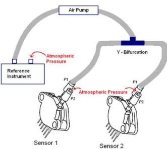
Inside the signal acquisition module, the manovacuometer employs two differential sensors (figure 2), one for PImax and other for PEmax. The main features of the sensor can be found in table 1 (Freescale, 2004). Nevertheless, it is important to emphasize that pressure on side P1 must be always higher than on P2. Thus, sensor 1 measures PEmax (PE applied on P1) and sensor 2 measures PImax (PI applied on P2). The sensors have a pressure range from 0 up to 50 kPa.
Figure 1: Digital manovacuometer developed by NEPEB (Núcleo de Estudos e Pesquisa em Engenharia Biomédica). On the left, the pressure signal acquisition module; on the right, the A/D converter module.
Table 1: Operating characteristics of the sensor MPX5050.
Characteristic Symbol Minimum Typical Maximum Unit
Pressure Range PCP 0 – 50 kPa
Supply Voltage VF 4.75 5.00 5.25 Vdc
Supply Current Io – 7.0 10.0 mAdc
Minimum Pressure Offset (0 to 85oC)
Voff 0.088 0.20 0.313 Vdc @VF = 5.0 Volts
Full Scale Output (0 to 85oC)
VF SO 4.587 4.70 4.813 Vdc
@VF = 5.0 Volts
Full Scale Span (0 to 85oC)
VF SS – 4.5 – Vdc
@VF = 5.0 Volts
Accuracy – – – +/−2.5% VF SS
Sensitivity V/P – 90 – mV/kPa
Response Time tR – 1.0 – ms
Output Source Current at Full Scale Output Io+ – 0.1 – mAdc
Warm-Up Time – – 20 – ms
Offset Stability – – +/−0.5 – %VF SS
13 channels, 10 bits A/D converter, emulating the RS232 communication protocol through an USB interface (Microchip, 2007b; Microchip, 2007c). As in Olson (1998), the signal frequency range of respiratory flow is from 0 to 40 Hz. Thus, a Butterworth low-pass, anti-aliasing filter, 40 Hz cutoff frequency (order 2) was used for a sampling frequency of 1 kHz (Oliveira Júnioret alli, 2008).
2.2
Calibration procedure
Figure 2: Schematic implementation for prototype calibration
Table 2: Pressure values applied to prototype.
Pressure (kPa) 4.0 9.3 12.0 13.3 20.0 26.7 33.3 40.0 46.7 53.3 60.0 –
value and them decreased to 0 kPa. Each value has to be applied for approximately five seconds, and after the average voltage is measured at the output of the manovacuometer. The calibration points are showed in table 3. Two extra points, whose pressure value is higher than superior range value (50 kPa), were inserted into the set of calibration points to check the start region of non-linearity on the curve. Alongside with the data acquisition to plot the calibration curves for both sensors, tests were implemented to find out: i) the maximum indication error and ii) the sensor hysteresis.
Table 3: Reference pressure, output voltage values and associated uncertainties – sensor 2 (rising curve).
Pr(kPa) uPr(kPa) Vm(V) uVm(V)
4.0 0.1 0.458 0.002 9.3 0.1 0.926 0.007 12.0 0.1 1.175 0.002 13.3 0.1 1.291 0.004 20.0 0.1 1.890 0.004 26.7 0.1 2.496 0.005 33.3 0.1 3.097 0.005 40.0 0.1 3.709 0.004 46.7 0.1 4.333 0.003 53.3 0.1 4.941 0.005
The measurement procedure was performed four times for each sensor, and both the average rising and the average fall curves of the output voltage versus applied pressure were obtained for each sensor. In order to check for drifting two groups of measurement were done distant six month in time, the first group collected in April 2007 and the second collected in October 2007.
2.3
Estimation of calibration curve of the
digital manovacuometer
To implement the linear fitting for the calibration points, the method of weighted least squares – WLS was used (Lira, 2002; GUM, 2003; Mathioulakis and Belessiotis, 2000; Presset alii, 1996). It was chosen to obtain curve fitting for the average rising and for the average fall curves for each sensor (Ferreiraet alli, 2008a).
2.4
Evaluation
of
measurement
uncertainty
The measurement uncertainty for that prototype was determined according to the “Guide to the Expression of Uncertainty in Measurement” – GUM (GUM, 2003). Two mathematical measurement models were developed (GUM, 2003; Lira, 2002; Mathioulakis and Belessiotis, 2000): i) using the datasheet expression (manufacturer calibration curve, presented in Freescale (2004); ii) using the expression (calibration curve) estimated with the experimental data employing the weighted least squares (WLS) fitting.
Figure 3: Mean transfer function for sensor 1.
2.5
Calibrated measurement reference
3
RESULTS
3.1
First group of collected data
The prototype transfer function curve obtained with the WLS fitting will be determined first. Then, the evaluation of the measurement uncertainty will be done for both measurement models.
3.1.1 Prototype Transfer Function Curve Using WLS Fitting
The output voltageVm versus input pressurePrcurves are
shown in figure 3 (increasing input pressure and decreasing input pressure – rising and fall) for sensor 1 of the NEPEB manovacuometer. Similar curves were obtained for sensor 2. Observing this figure, it is noticed that linearity is present up to Pr = 53.3kP a. Thus, calculations was carried
out also considering the calibration point with this pressure value. The calibration point with pressure equal to 60 kPa was discarded.
Taking the experimental data (Vm ×Pr) up to 53.3 kPa
(J = 10 points) and employing a curve fitting method, the transfer function relating the voltage indication at manovacuometer display and the input pressure can be described with a linear model (Mathioulakis and Belessiotis, 2000):
Prc=b+aVm (1)
where Prc is the pressure in kiloPascal that corresponds
to the voltage Vm, indicated at the display of the NEPEB
manovacuometer;ais the slope of the fitted curve andbis its intercept (Ferreira etalli,2008a). The correspondent values indicated by the pressure measurement standard instrument, Prassociated toVmof sensor 2 are given in table 3.
As mentioned earlier, any measurement result is composed by a numeric value indicating the quantity estimated value and by the measurement uncertainty. Frequently, measurement uncertainty is obtained using a mathematical measurement model, which is that function which contains every quantity, including all corrections and correction factors, that can contribute with a significant component of uncertainty to the measurement result.
In the case of the NEPEB manovacuometer, among the uncertainty components, relevant to the measurement result, one should include the contribution obtained with the WLS fitting method. The uncertaintyuP rwas evaluated using the
related standard expanded uncertainty (uP r = 0.03%/2,
multiplied by Pr) and the resolution of the display device
of the reference manovacuometer. On the other hand,
the uncertainty uV m was estimated based on fluctuation
of the repeated readings (prototype output voltage) in each calibration point (Mathioulakis and Belessiotis, 2000) correspondent to the standard deviation of the mean, uV
(type A uncertainty), that is:
uV m=uV =
sV
√
n (2)
where sV corresponds to standard deviation of the voltage
values for the four rising (falling) curves and n is the number of points(n = 4, in that case).
The mathematics of linear regression fitting using weighted least squares is described with more details in Lira (2002), Mathioulakis and Belessiotis (2000) and Presset alii(1996). The slope a and the intercept b as well as the associated uncertaintiesuaeubcan be obtained from:
KT·K·C=KT·L (3)
whereCis a vector whose elements are the fitted coefficients a and b; and Q = (KT · L)−1) is a matrix whose
diagonal elements are the variances of a(q2,2)andb(q1,1).
The off-diagonal elementsq1,2 = q2,1are the covariances
between these parameters. K is the matrix with J ×2
components: K=
kJ,1 kJ,2 · · · · · ·
k1,1 k2,2
, where kj,1=w1j and kj,2=Vwmij
(4)
Lis the vector:
L=
Pr1/
w1 · · ·
PrJ/
wJ (5)
It is worthwhile to observe that the elements ofKandLare weighted inversely as pounds wj. Solving (3), one obtains
Table 4: Values for the parameters a and b and their uncertaintiesuaandub.
Sensor 1 Sensor 2
Rising Fall Rising Fall
a(kPa/V) 10.9756 10.9702 10.9994 10.9913
ua (kPa/V) 0.0230 0.0221 0.0238 0.0219
b (kPa) -0.5570 -0.4865 -0.8903 -0.8190
ub (kPa) 0.0638 0.0619 0.0668 0.0621
Cov(b, a) (kPa/V)
−1.25×10⁻³ −1.16×10⁻³ −1.36×10⁻³ −1.16×10⁻³
Table 5: Birge Ratio for sensor 1 and sensor 2 curves – data collected in April 2007.
Birge Sensor 1 Sensor 2
Ratio Rising Fall Rising Fall Bi 1.0755 1.0716 1.0412 1.0869
3.1.1.1 Consistency Analysis
In the literature, it is emphasized the importance to verify the consistency analysis between the fitted model and experimental data which is implemented by using the so-called chi-squared test (Lira, 2002; Cox and Harris, 2006). The test provides a number, the Birge Ratio (Bi), which one expects to be approximately equal to one. The value of Bi for the adjusted models and experimental data collected in April 2007 are indicated in table 5.
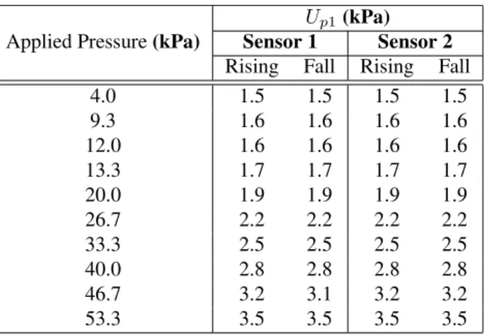
Table 6: Expanded uncertainty for all calibration points using the model obtained by the datasheet equation.
Applied Pressure(kPa)
Up1(kPa) Sensor 1 Sensor 2
Rising Fall Rising Fall 4.0 1.5 1.5 1.5 1.5 9.3 1.6 1.6 1.6 1.6 12.0 1.6 1.6 1.6 1.6 13.3 1.7 1.7 1.7 1.7 20.0 1.9 1.9 1.9 1.9 26.7 2.2 2.2 2.2 2.2 33.3 2.5 2.5 2.5 2.5 40.0 2.8 2.8 2.8 2.8 46.7 3.2 3.1 3.2 3.2 53.3 3.5 3.5 3.5 3.5
3.1.2 Evaluation of the Measurement Uncertainty
In order to exemplify the calculations of the measuring uncertainty in relation to a calibration point, the pressure value of 26.7 kPa of the rising curve of the sensor 2 (table 3) was arbitrarily chosen. For this point, the average output voltage isVm = 2.496V (standard deviation,sv, equals to
Figure 4: Calibration points and estimated curve by the model based on datasheet equation (Eq.) and associated uncertainties for sensor 2 (rising). Calibration points (+), estimated curve(Pe)resulting from (8) and estimated curve associated to expanded uncertainty (Pe+Up1andPe−Up1).
0.010 V).
According to GUM (2003), initially one must establish the functional relationshipf, relating the measurandY and the
input quantities,X1, X2, . . . , XN,:
Y=f(X1, X2, ..., XN) (6)
3.1.2.1 Evaluation of Uncertainty Using the Datasheet Expression
To build the first model to calculate the measurement uncertainty, the following equation found in the sensor datasheet was used (Freescale, 2004):
VS =VF(P×0.018 + 0.04) (7)
whereVS is the sensor output voltage, VF is sensor supply
voltage, and P is the pressure applied to sensor. Also according to the sensor datasheet, the expression above is valid for a range of temperature from 0 to85oC, but it was
employed at laboratory with controlled temperature (room temperature). From (7) one obtains:
P = 500 (VS−0.04VF) 9VF
(8)
Hence, (8) permits to calculate the pressure associated to the sensor output voltage. Calculations of uncertaints of input quantities of above equation take account type B uncertaints. Type B uncertainty (Ferrero and Salicone, 2006) is estimated considering sensor accuracy, uE, and supply voltage
variability,uF A, and offset stability (drift),uD:
uE =
0.1125 √
3 = 0.0650V uF A = 0.25
√
3 = 0.1443V
The value of uD = 0.0225 V is inferred according to
indicated in table 1. It must be observed that the probability distribution was assumed as a uniform distribution foruE
anduF A.
Since the input quantities correlation was neglected, the application ofthe law of propagation of uncertaintiesto (8) implies, for this metrological model, the combined standard uncertainty as:
u2C1(P) =
∂P
∂VS
2
u2S +
∂P
∂VF
2
u2F (9)
where
uS =uE⇒uS = 0.0650V ,
u2F =u2F A+u2D⇒uF = 0.1461V ,
∂P ∂VS
= 500 9VF
= 11.1111kP a
V , ∂P
∂VF
=−5009VV2S
F
=−5.546kP a
V
The value ofVF used for calculations is the average value of
the supply voltage, equal to 5 V. Likewise, the average value is used forVS = Vm = 2.496 V. Thus, one obtains
uc1(P) = 1.1kP a.
The expanded standard uncertainty, Up1, was estimated
assuming a confidence interval (Ferrero and Salicone, 2006) equal to 95.45%. To evaluate the degrees of freedom,νef f,
the expression of Welch-Satterwaite (GUM, 2003) was used and the value is estimated as → ∞. Thus, the coverage factor isk1 = 2and so one obtains:
Up1=k1×uc1(P) = 2×1.1kP a= 2.2kP a
The expanded uncertainties for all calibration points (rising curve of the sensor 2) have been calculated inside the pressure range 1.5 – 3.5 kPa (table 6). Similar uncertainty range was calculated for remainder curves. In figure 4, the obtained experimental data (calibration points) and estimated pressure curves using information of the sensor datasheet are shown.
3.1.3 3.1.2.2 Evaluation of Uncertainty with Curve Fitting by Weighted Least Squares Method
The second proposed model to estimate uncertainty was built taking into account (1), based on the weighted least squares (WLS) linear adjustment (Mathioulakis and Belessiotis, 2000).
Calculation of the uncertaintyuP cassociated to calibration
points is also derived from application of the law of propagation of uncertaintiesto (1), resulting (Ferreiraet alli, 2008a):
uP c= a2u2V m+u2b+Vm2u2a+ 2VmCov(b, a)
1/2
(10)
where the uncertainty uV m is estimated considering the
type A uncertainty, uV, and the resolution of NEPEB
manovacuometer,uR:
uV =
sV
√
n=
0.010 √
4 = 0.005V
uR=
0.001 √
3 = 0.0006V
u2V m=u2V+u2R⇒uV m= 0.005V
Taking account these values as well as those of third column of table 4 and substituting in (10), results uP c = 0.0654kP a.
The standard combined uncertainty, in turn, was obtained by:
u2c2(P) =u2P c+u2Pr (11)
where, again, uP r = 0.1 kP a is the uncertainty
associated to reference instrument and is obtained by:uPr= r
0.03%
2 ×26.7 2
Thus, the standard combined uncertainty is estimated as uc2(P) = 0.1kP a.
Considering the confidence interval of 95.45%, likewise the first model, the effective number of degrees of freedom is νef f → ∞, indicating k2 = 2. Thus, the estimated
value for the standard expanded uncertainty is equal to Up2 = 0.2kP a.
The calculated expanded uncertainty for the others calibrations points of the rising curve of the sensor 2 and remainder curves was estimated about 0.2 to 0.3 kPa. In figure 5a, the obtained experimental data (calibration points) and estimated pressure curve by WLS are observed. In figure 5b, the curves were plotted on a differente scale, so that only two calibration points are shown.
(a)
(b)
Figure 5: (a) Calibration points and estimated curve by the model based on WLS and associated uncertainties for sensor 2 (rising). (b) Zoom nearbyPe = 30kP a: calibration points (+), estimated curve(Pe)resulting from linear adjustment and
estimated curve associated to expanded uncertainty (Pe+Up2
andPe−Up2).
3.2
Second group of collected data
The analysis implemented for the set of data collected six month after the first followed the same procedure carried out for the first. Great similarity with the first set of collected data was observed, and the calculated expanded uncertainty by WLS modeling was estimated to be about 0.3 to 0.5 kPa.
3.2.1 Consistency Analysis
The new values ofBifor the fitted models and experimental data collected six month after the first group are shown in table 7.
Table 7: Birge Ratio for sensor 1 and sensor 2 curves – data collected in October 2007.
Birge Ratio (Bi) Sensor 1 Sensor 2 Rising Fall Rising Fall
0.6949 0.6927 0.6877 0.8294
4
DISCUSSION
Calibration performed to the digital manovacuometer prototype developed in NEPEB indicates a strong repeatability of output voltage measurement of calibration curves. The maximum value obtained for the type A uncertainty was equal to 0.72% that is associated to the value ofVm = 0.926V, related to the set of data of April
2007, and 3.09%, associated to the valueVm = 0.412V,
related to data of October 2007.
Calculations of hysteresis were performed considering the rising and fall fitting curves for each sensor. The maximum absolute value obtained was equal to 0.0639 kPa (0.48%) for sensor 1 and 0.0842 kPa (0.16%) for sensor 2 (data of April 2007). For the set of data collected in October 2007, these values were 0.0830 kPa (0.21%) for sensor 1 and 0.1017 kPa (0.19%) for sensor 2. These values are much lower than the value established by INMETRO for sphygmomanometers with aneroid manometer (0.5 kPa). In the same way, when the linear region is considered, it is noticed that the results obtained in maximum indication error test (≤ 0.1687 kPa for data of Apr/2007 and≤ 0.2313 kPa for data of Oct/2007) are also inside the tolerance range determined by INMETRO for this equipment (0.4 kPa).
manufacturer sensor especification.
Considering the calibration fitted curves by WLS, according to consistency analysis verified (Lira, 2002), non-conformities between data and models were not observed: calculated values for the Birge ratio is near to unity (tables 5 e 7).
5
CONCLUSION
The calibration model proposed in this work was employed to obtain the calibration curves and to evaluate the measurement uncertainties for a digital manovacuometer prototype (developed in NEPEB). It is expected that this work can be used by the technical staff from the hospitals and alike to quality measurement during physiotherapeutic diagnosis or treatment.
Results estimated by the two proposed models to calculate the measurement uncertainties show the range of values evaluated by WLS inside the range of values evaluated by information listed in the sensor datasheet. By the second model, designed using weighted least squares adjustment (WLS) at the laboratory, the values range for expanded uncertainty extends from 0.2 up to 0.5 kPa. In turn, the values range observed for the model built using information of sensor datasheet extends from 1.5 up to 3.5 kPa. Therefore, the metrological analysis implemented here shows adequacy for digital manovacuometer prototype use.
The calibration procedure has permitted to know about the reliability of the DM to measure maximum respiratory pressure. In future works, the digital manovacuometer will be used in clinical application and periodicity between calibrations will be checked. The small variation observed when comparing the two set of data acquired months apart for the values of ucertainty calculated by WLS modeling shows, clearly, the demand to perform this cheking. Yet, others uncertainty sources could be evaluated in the models to assess the impact on the results like those related to the low-pass filter, A/D converter and temperature variation.
ACKNOWLEDGMENTS
To FAPEMIG and CNPq for financial support.
To CETEL/SENAI/FIEMG represented for Luiz Henrique, Marcus Vinicius and Reiner that lent the laboratory and reference manovacuometer for the measurements.
REFERENCES
Black, L.F. and R.E. Hyatt (1969). Maximal respiratory pressures: normal values and relationship to age and
sex.Am. Rev. Respir. Dis.99(5), pp. 696-702. Cox, M.G. and P.M. Harris (2006). Measurement
uncertainty and traceability.Meas. Sci. Technol.(Jan.),
17, pp. 533-540.
Ferreira, J. L. (2008). Metrology applied to a digital maximum respiratory pressures measuring system (free translation). M.S. Thesis. Dept. of Electrical Engineering. Universidade Federal de Minas Gerais – UFMG, Belo Horizonte, Brazil.
Ferreira, J.L., N.C. Pereira, M. Oliveira Júnior, J.L. Silva, R.R. Britto, V.F. Parreira, F.H.Vasconcelos, C.J. Tierra-Criollo (2008a). Application of weighted least squares to calibrate a digital system for measuring the respiratory pressures. Proc. of Biodevices: 1st
International Conference on Biomedical Electronics and Devices, Funchal, Portugal, v. 1, pp. 220-223. Ferrero, A., and S. Salicone (2006). Measurement
Uncertainty. IEEE Instrum. Meas. Mag., (Jun.), pp. 44-51.
Freescale (2004). Sensor data book. Available: <http:www.freescale.com>Access in: Nov. 03 2005. GUM (2003). Guide to the expression of uncertainty in
measurement. 3rd Brazilian ed. ABNT, INMETRO, Rio de Janeiro.
INMETRO (2007). Homepage of INMETRO. Available: <http://www.inmetro.gov.br>. Access in: Aug. 20 2007.
INMETRO (1997). Procedure for verification of the sphygmomanometers with aneroid manometer (free translation). INMETRO, Rio de Janeiro.
Lira, I. (2002) Evaluating the measurement uncertainty: fundamentals and practical guidance. IoP, Bristol and Philadelphia.
Mathioulakis, E. and V. Belessiotis (2000). Uncertainty and traceability in calibration by comparision. Meas. Sci. Technol.(Mar.),11, pp. 771-775.
Microchip (2007a). About Microchip USB PIC (PIC18F2550, PIC18F4550...). Available: < http :
//pic18f usb.online.f r/wiki/wikka.php?wakka =
W ikiHome > .Access in: May 01 2007.
Microchip (2007c). Emulating RS-232 over USB with PIC18F4550 - Microchip Technology Inc. Available: <http:// techtrain.microchip.com/ webseminars/ documents/ EmulatingRS-232overUSB_121004.pdf>. Access in: May 01 2007.
Oliveira Júnior, M., F. Provenzano, P.A. Moraes Xavier, N.C. Pereira, D. Montemezzo, C.J. Tierra-Criollo, V.F. Parreira, R.R. Britto (2008). Medidor digital de pressões respiratórias. Proc. of 21o. Congresso Brasileiro de Engenharia Biomédica, Salvador, Brazil, pp. 741 – 744.
Olson, W.H. (1998). Basic concepts of medical instrumentation. In J.G. Webster (Ed.), Medical instrumentation: application and design.3rd ed. Wiley, New York.
Parvis, M. and A. Vallan (2002). Medical measurements and uncertainties. IEEE Instrum. Meas. Mag. (Jun.), pp. 12 – 17.
Press, W.H., S.A. Teukolsky, W.T. Vetterling and B.P. Flannery (1996). Numerical recipes in C: the art of scientific computing. 2nd ed. Cambridge, University Press Cambridge.
Silva, J. L. (2006). Development of a digital system for measuring maximum respiratory pressures (free translation). Graduating Final Work of Control and Automation Course, Available: School of Eng. Library, Universidade Fedral de Minas Gerais – UFMG, Belo Horizonte, Brazil.