KINEMATIC CONTROL OF CONSTRAINED ROBOTIC SYSTEMS
Gustavo M. Freitas
∗ [email protected]Antonio C. Leite
∗ [email protected]Fernando Lizarralde
∗∗Department of Electrical Engineering - COPPE
Federal University of Rio de Janeiro Rio de Janeiro, RJ, Brazil
RESUMO
Controle de Sistemas Robóticos com Restrições Cinemáticas
Este artigo considera o problema de controle de pos-tura para sistemas robóticos com restrições cinemáti-cas. A ideia principal é considerar as restrições cine-máticas dos mecanismos a partir de suas equações es-truturais, ao invés de usar explicitamente a equação de restrição. Um estudo de caso para robôs paralelos e robôs cooperativos é discutido baseado nos conceitos de cinemática direta, cinemática diferencial, singularidades e controle cinemático. Resultados de simulação, obti-dos a partir de um mecanismo Four-Bar linkage, uma plataforma de Gough-Stewart planar e dois robôs coo-perativos, ilustram a aplicabilidade e versatilidade da metodologia proposta.
PALAVRAS-CHAVE: robôs paralelos, robôs redundantes, coordenação multi-rôbos, singularidades cinemáticas .
ABSTRACT
This paper addresses the posture control problem for robotic systems subject to kinematic constraints. The key idea is to consider the kinematic constraints of the mechanisms from their structure equations, instead of explicitly using the constraint equations. A case study
Artigo submetido em 10/03/2011 (Id.: 01293) Revisado em 27/05/2011
Aceito sob recomendação do Editor Associado Prof. Carlos Roberto Minussi
for parallel robots and cooperating redundant robots is discussed based on the following concepts: forward matics, differential kinematics, singularities and kine-matic control. Simulations results, obtained with a Four-Bar linkage mechanism, a planar Gough-Stewart platform and two cooperating robots, illustrate the ap-plicability and versatility of the proposed methodology.
KEYWORDS: Parallel robots, redundant robots, multi-robot coordination, kinematic singularities.
1
INTRODUCTION
scaling. These drawbacks could be overcome by the use
of parallel robots to increase rigidity, redundant robots
or mobile manipulators (manipulators mounted on a
mobile robot,e.g.,remotely operated vehicles, wheeled robots) to augment the system workspace and/or avoid singularities in order to accomplish the task of interest (Murray et al., 1994).
Parallel robots provide a rigid connection between the base structure and the payload to be handled by the end-effector, with positioning accuracy superior to the one obtained by serial chain manipulators (Merlet, 1993; Merlet and Gosselin, 2008). The main disadvantages of using parallel robots are: workspace limitation, more complex forward kinematics maps and more involved singularity analysis (Wen and O’Brien, 2003; O’Brien et al., 2006; Simas et al., 2009). For instance, in contrast to serial chain manipulators, the singularities in parallel mechanisms may have different characteristics.
In this context, the singularities can be classified into three basic types (Gosselin and Angeles, 1990; Liu et al., 2003):
(i) configuration space singularities: when the rank of the structure equations drops and, thus, the end-effector loses the ability to move instantaneously in some directions;
(ii) end-effector singularities: when the end-effector loses degrees of freedom (DOF), that is, the mo-tion of the active joints can result in no momo-tion of the end-effector;
(iii) actuator singularities: when the actuator of the manipulator or the active joints cannot produce end-effector forces and torques in some directions.
The kinematic and dynamic control problems for paral-lel robots are considered in (Kövecses et al., 2003; Cheng et al., 2003; Rosario et al., 2007) and an autonomous control approach to reach the dynamic limits of parallel mechanisms is presented in (Pietsch et al., 2005).
Redundant manipulators have more degrees of freedom1
that those strictly necessary to perform a given task. Redundancy is therefore a relative concept for a robot manipulator, depending on the particular type of task to be executed. For example, six DOF are necessary for positioning and orienting a robot end-effector, thus a6 -DOF manipulator is considered non-redundant. How-ever, if only the positioning task is of concern, the same arm becomes redundant. The extra degrees of freedom provide more dexterity to the robot structure, and it can be used to avoid kinematic singularities
and collision with obstacles, as well as to optimize the robot motion with respect to a cost function (e.g.,joint torque energy). Furthermore, considering the pres-ence of mechanical joint limits, redundant manipula-tors can also be used to increase the robot workspace (Siciliano, 1990; Chiaverini et al., 2008). In general, multiple cooperating robot arms and mobile manipu-lators, for instance, belong to the class of redundant robots (Caccavale and Uchiyama, 2008).
The coordination of multiple robots is an essential activ-ity in several industrial applications, such as assembly and manufacturing tasks, where multiple robotic arms are often grasping an object in contact with the envi-ronment. Typical examples include: deburring, con-tour following, grinding, machining, painting, polish-ing and object alignpolish-ing (Namvar and Aghili, 2005) or even robot dexterous hands (Caurin and Pedro, 2009). In this framework, a study of the differential kinemat-ics and manipulability indexes for multiple cooperating robot arms with unactuated joints is presented in (Wen and Wilfinger, 1999; Bicchi and Prattichizzo, 2000). Ad-vanced motion and force control of cooperative robotics manipulators with passive joint are considered in (Tinos et al., 2006; Pazelli et al., 2011). A screw-based system-atic method to derive the relative Jacobian for two co-operating robots is developed in the recently published work (Ribeiro et al., 2008; Simas et al., 2009).
Motivated by several applications to parallel robots and redundant manipulators, this paper provides a control methodology for robotic systems under kinematic con-straints based on a novel proposed method (Wen and O’Brien, 2003). The key idea is to consider the kine-matic constraints of these mechanisms from their struc-ture equations, rather than explicitly using the con-straint equations. The major advantage of this method-ology is its applicability and versatility when different robotic systems are considered. Simulation results are obtained from the kinematic models of a Four-Bar link-age mechanism, a planar Gough-Stewart platform and two cooperating robots.
Terminology and Notation
In this work, the following notation, definition and as-sumptions will be adopted:
¯
Ea = [⃗xa ⃗ya ⃗za ]denotes the orthonormal frame
aand⃗xa, ⃗ya, ⃗zadenote the unit vectors of the frame axes.
1
For a given vectorx∈Rn, its elements are denoted byxi fori= 1· · ·n, that is,x= [x1 x2 · · · xn]T.
ne : number of effective degrees of freedom of the mechanism2.
nt:number of degrees of freedom required to per-form a task.
Definition 1 A robotic system can be classified as: (i) non-redundant: ne≤nt; (ii) redundant: ne> nt.
Assumption 1 For an open-chain mechanism consti-tuted by i+ 1 links connected by n joints, where the link0is fixed, each joint provides a single degree of mo-bility to the mechanism structure, andn=i.
Assumption 2 For a closed-chain mechanism consti-tuted by i+ 1 links, the number of joints n must be greater thani. In particular, the number of closed loops is equal ton−i.
2
CONSTRAINED ROBOTIC SYSTEMS
This section considers the kinematics of the closed-chain robotic systems subject to kinematic constraints on ve-locity. The general methodology to derive the forward kinematics and the differential kinematics equations for constraint-based robotics systems is to open the loop of the mechanism, propagate the kinematics along the branches and add the kinematic constraints.
Let p∈ (R)3 be the position of the end-effector frame ¯
EE with respect to the robot base frame E0¯ , and R∈
SO(3)the orientation of the end-effector frameE¯Ewith respect to the robot base frame E¯0 3. In this context,
the posture (position and orientation) of the robot end-effector can be obtained from the forward kinematics map as
{p, R}=k(θ), (1) wherek(·) :Rn7→ {R3, SO(3)} is a non-linear mapping andθ∈Rnis the vector of joint variables (or generalized coordinates) expressed in the unconstrained configura-tion space Q. The vector of active joints (or actuated joints) is denoted byθa∈Rna, whereas the vector of pas-sive joints (or unactuated joints) is denoted byθp∈Rnp, where n=na+np. Then, we can rearrange the vector of joint angles, such that,θT= [θT
a θpT]. The kinematic 2
The effective degrees of freedom for a mechanism can be calculate by means of the Gruebler’s formula, provided that the constraints imposed by the joints are independent (Murray et al., 1994).
3
Special Orthogonal Group SO(3) = {R∈ R3×3
:RTR=
I, det(R) = 1}
constraints can be locally represented as algebraic con-straints in the configuration spaceQby
c(θ) = 0, (2)
wherec(·) :Rn7→Rr. Then, the mechanism hasn e=n−r effective degrees of freedom and the following assump-tion is considered:
Assumption 3 The number of active joints is equal to the effective degrees of freedom, that is,na=ne.
Note that, the constraint described in (2) is an example of holonomic constraint. In general, a constraint is said to be holonomic if it restricts the motion of the system to a smooth hypersurface in the configuration spaceQ
(Murray et al., 1994).
Now, considering that the constraint can be written in terms of the joints velocity vectors, we have
Jc(θ) ˙θ= 0, (3) where Jc=∂c∂θ(θ)∈Rr×n is named the constraint Jaco-bian.
On the other hand, the end-effector velocity v, com-posed by the linear velocity p˙ and the angular velocity
ω (defined asR˙ =ω×R(Murray et al., 1994)), can be related with the velocityθ˙ by
v=
[
˙ p ω
]
=Jm(θ) ˙θ , (4)
whereJm∈Rn×nis the manipulator geometric Jacobian (Siciliano et al., 2008).
Partition the Jacobians Jc and Jm according to the dimension of active-passive joint variables, θa and θp, we have Jc= [Jca Jcp] and Jm= [Jma Jmp]. Then, without loss of generality, the equations (3) and (4) can be rewritten as (Wen and O’Brien, 2003; O’Brien et al., 2006):
0 =Jcaθ˙a + Jcpθ˙p, (5)
v =Jma θ˙a + Jmpθ˙p, (6) where Jca∈Rnp×na, Jcp∈Rnp×np, Jma∈Rm×na and
Jmp∈Rm×np.
From (5), θ˙p can be calculated in terms of the active joints as
˙
Substituting (7) into (6), the differential kinematics equation can be rewritten as
v= (Jma−JmpJcp−1Jca)
| {z }
¯
J(θa,θp)
˙
θa, (8)
whereJ¯∈R6×n−r. In the case thatJ¯be invertible, the control law is similar to the kinematic control case of the serial chain manipulator. For example, for a given desired positionpd(t), a proportional control plus feed-forward could be proposed:
u= ˙θa= ¯Jp(θa)† [K (pd−p) + ˙pd] (9) where K > 0 is the controller gain matrix and J¯p ∈
R3×n−r is the partition of J¯ relating the contribution of the active joint velocity θ˙a to the end-effector lin-ear velocity p˙. Note that a PI controller could also be used, however this controller only guarantees zero steady state error for step-typepd. For the orientation control, a representation of the end-effector orientation
R ∈SO(3) should be considered, e.g. unit quaternion (Murray et al., 1994).
From the analysis of the equation (8), we conclude that a singularity in J¯occurs when the rank of matrix Jcp drops. In this case, implies that there is internal motion of the joints, even when the active joints are locked. This type of singularity is named byunstable singularity or
actuator singularity(see (Wen and O’Brien, 2003; Kim
et al., 2001) for a detailed discussion).
3
PARALLEL MANIPULATORS
In this section, a planar Four-Bar linkage mechanism is used to illustrate the posture control problem for paral-lel manipulators. In sequence, the presented methodol-ogy is applied to a planar Gough-Stewart platform. A parallel manipulator is a closed-chain mechanism with end-effector and fixed base, composed by the union of two open kinematic chains at least. Parallel tors can present advantages over open-chain manipula-tors in terms of (i) rigidity of the mechanism, due to the presence of two or more closed chains, and(ii) actu-ators allocation, since in general onlyne actuators are necessary (Merlet and Gosselin, 2008).
3.1
Kinematic singularities
The singularities of the parallel mechanisms can be clas-sified into(i) serial or end-effector singularity and (ii)
parallel or actuator singularity. When both singularities occur simultaneously, they are named structural singu-larity (Gosselin and Angeles, 1990).
In a serial singular configuration, the joints can have a nonzero velocity while the mechanism is at rest. In this case, the end-effector loses degrees of freedom in the task space. On the other hand, in a parallel sin-gular configuration there exist nonzero velocities of the mechanism for which the joint velocities are null, and in this case the end-effector gains some degrees of freedom in the task space. A parallel singularity is especially im-portant for parallel mechanisms since it corresponds to configurations where the robot loses the controlability. Moreover, excessive forces can occur in the vicinity of singular poses and consequently to lead the breakdown of robot parts.
Finally, it is worth to mention that in some cases, sin-gular configurations can be useful. For instance, high amplification factors between the actuated joint motion and the end-effector motion can be essential for improv-ing the sensitivity along some measurements directions for a parallel robot used as a force sensor, or for accurate positioning devices with very small workspace (Merlet and Gosselin, 2008)
3.2
Planar Four-Bar linkage mechanism
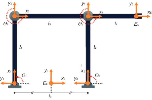
The considered Four-Bar linkage mechanism is formed by a single closed kinematic chain, composed by the union of two open chains (Figure 1). The mechani-cal structure consists of four rigid bodies connected by means of revolute joints, where the active joint isθa=θ1 and the passive joints areθp= [θ2 θ3 θ4]T. Note that, links l3 andl4 compose one link.
x1
x3
x2
x0
x4 xE
y0
y1 y2
y3 y4 yE
!2 !4 !3
!1
E0
EE
l1
l1
l3
l2
l4
l0
l2
l2
Figure 1: Planar Four-Bar linkage mechanism.
appli-cations as machine components and tools, automotive suspensions and bolt cutters.
3.2.1 Forward kinematics
The forward kinematics map of a parallel manipulator is described by the posture (position and orientation) of the end-effector frame E¯E with respect to the base frameE0¯ , derived for each kinematic chain. For parallel mechanisms, the forward kinematics problem is usually much more complex than the inverse kinematics prob-lem, due to the closed loop nature of the mechanism. In order to obtain the forward kinematic, an appropri-ate frame E¯i for i = 1,· · · , l is attached to i-th link. Thus, the structure equations (or loop equations) of the Four-Bar linkage mechanism are given by:
p = p01+p13+p3E
| {z }
chain 1
=p02+p24+p4E
| {z }
chain 2
, (10)
ϕ = θ1+θ3
| {z } chain 1
=θ2+θ4
| {z } chain 2
, (11)
whereϕ∈Rrepresents the end-effector orientation (for the planar case the orientationRis an elementary rota-tion about thezaxis,i.e. R=Rz(ϕ)) andpij∈R3is the position vector of the origin of frameE¯j with respect to the origin of the frame E¯i. The structure equations of the mechanism introduce constraints between the joint angles of the manipulator. Considering the planar case, where p∈R2 and ϕ∈R, equations (10) and (11) corre-spond to r= 3 constraints. Thus, the Four-Bar linkage mechanism withn= 4joints hasne=n−r= 1effective degrees of freedom. This result can also be obtained by using the Gruebler’s formula for planar motions (Murray et al., 1994).
Remark 1 For parallel mechanisms, the number of passive joints is always equal to the number of con-straints, that is, np = r. Thus, the vector of joint variables θ∈Rn can be partitioned as (θa, θp), where
θa∈Rn−r are the active joint variables andθp∈Rrare the passive joint variables.
The kinematic constraints of the mechanism allow us to control the end-effector orientation by specifying only the angular position of the active jointθa=θ1, and the other joint variables must take on values in order to satisfy the structure equations. Thus, the passive joints
θp∈R3 can be obtained as a function of active joints
θa∈R by means of the forward kinematics equation of
the mechanism, by using the chain1
p=p01+p13+p3E =−
l0
2 ⃗x0+l1R01(θ1)⃗x0+ (l3+l4)R01(θ1)R13(θ3)⃗x0, (12) or the chain2
p=p02+p24+p4E =
l0
2 ⃗x0+l2R02(θ2)⃗x0+ l4R02(θ2)R24(θ4)⃗x0, (13)
where Rij(θi)∈SO(3) denotes the orientation of the frame E¯j with respect to the frame E¯i. Note that, in this case, Rij is an elementary rotation matrix by an angleθi about the axiszof the frameE¯i. After the use of geometric and algebraic identities, the passive joints
θp are obtained by
θ2=π−arccos
(
l2
0−l21+ld2
2l0ld )
−arccos
(
l2
2−l23+l2d
2l2ld )
,
θ3=π+ arccos
(
l21−l20+ld2
2l1ld )
+ arccos
(
l32−l22+l2d
2l3ld )
,
θ4= 2π−arccos
(
l2
2+l32−l2d
2l2l3
)
,
where
ld2=l20+l12−2lol1cos(θ1).
In the case thatl3 =l0 andl1=l2, there always exists solution forθ3 and we has thatθ2=θ1andθ3=θ4. Now, it is possible to obtain the end-effector position from (12) or (13), as well as the end-effector orientation from (11), in terms of the active jointθa=θ1.
Remark 2 A more direct technique to solve the in-verse kinematics problem and obtain the passive joint variables θp is to apply the methods based on Paden-Kahan subproblems, in particular the subproblems 1
and 3 (Murray et al., 1994), which are geometrically meaningful and numerically stable.
3.2.2 Differential kinematics
Analogously, the differential kinematics of a parallel ma-nipulator is computed by considering the various open kinematic chains that compose the mechanism struc-ture. The end-effector velocity v∈R3 can be obtained from the time derivative of structure equations, result-ing in a Jacobian matrix for each serial chain
v=S J1
[ ˙
θ1 ˙ θ3
]
=S J2
[ ˙
θ2 ˙ θ4
]
whereS∈R3×6 is a selection matrix given by:
S=
1 0 0 0 0 0 0 1 0 0 0 0 0 0 0 0 0 1
, (15)
and the Jacobian matricesJ1∈R6×2andJ2∈R6×2are4:
J1 =
[
⃗
z0×p1E ⃗z0×p3E
⃗
z0 ⃗z0
]
, (16)
J2 =
[
⃗
z0×p2E ⃗z0×p4E
⃗
z0 ⃗z0
]
, (17)
with
p1E = l1R01(θ1)⃗x0+p3E, (18)
p2E = l2R02(θ2)⃗x0+p4E, (19)
p3E = (l3+l4)R01(θ1)R13(θ3)⃗x0, (20)
p4E = l4R02(θ2)R24(θ4)⃗x0. (21) The Jacobian of the mechanism can be rewritten in a more usual form, stacking the Jacobian of each open chain:
[
S J1 0 0 S J2
]
| {z }
J
˙ θ1
˙ θ3
˙ θ2
˙ θ4
| {z }
˙
θ
=
[
I I
]
| {z } A
v , (22)
or equivalently
J θ˙=A v , (23) where the matrixA∈R6×3has full column rank. Using
this notation, it is possible obtain the constraint Jaco-bianJc∈R3×4and the manipulator JacobianJm∈R3×4 by means of:
Jc = ˜A J , Jm=A†J , (24) where Ae ∈ R3×6 is the annihilator of A, such that,
e
A A= 0, and A† ∈ R3×6 is the pseudo-inverse of A,
such that A†A=I. A possible choice is Ae= [I −I] andA† = [I 0]. From (8), J¯∈R3×1can be calculated
byJ¯=Jma−JmpJcp−1Jca.
3.2.3 Kinematic control
In this section, the kinematic control approach is used to modify the posture of the Four-Bar linkage mecha-nism in order to perform a task of interest. Here, we assume that the control objective is to drive the cur-rent end-effector orientationϕto a desired time-varying orientationϕd(t), that is,
ϕ→ϕd(t), eϕ=ϕd(t)−ϕ→0, (25) 4
×denotes the vector cross product.
where eϕ∈Ris the orientation error.
The control scheme to be designed has to command the velocity of the active joint θ˙a= ˙θ1 in order to achieve the control objective (25). Then, using a proportional control law plus feedforward action
u= ˙θa= ( ¯J3)−1(kϕeϕ+ ˙ϕd), (26) where J3¯ is the third element of J¯and the orientation error dynamics is governed bye˙ϕ+kϕeϕ= 0, provided that the mechanism motions are away from singular con-figurations. Hence, by a proper choice ofkϕas a positive constant implies that limt→∞eϕ(t) = 0.
3.3
Planar Gough-Stewart platform
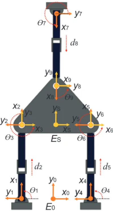
Another usual example of parallel mechanisms is the Gough-Stewart platform. Typically, some applications of this structure include: aircraft flight simulators, an-tennas and telescopes positioning systems, machine tool and crane technologies, and orthopedic surgery. In this section, we consider a planar version of the Gough-Stewart platform (Figure 2). The mechanical structure is composed by the union of three open chains and has nine joints, where three prismatic joints are active
θa = [d2 d5 d8]T, and six revolute joints are passive
θp = [θ1 θ3 θ4 θ6 θ7 θ9]T. We can obtain the effec-tive degrees of freedom for this mechanism by apply-ing the Gruebler’s formula for planar motions (Murray et al., 1994):
ne= 3(i−n) + n ∑
j=1
fi= 3, (27)
whereiis the number of mobile links in the mechanism,
nis the number of joints andfiis the number of degrees of freedom for thei-thjoint. From (27), we conclude that the mechanism has three effective degrees of freedom, which allow us to control the position and orientation of the platform respectively, in order to perform planar positioning tasks.
3.3.1 Forward kinematics
x
0y
0 !1E
0!4
x
4y
4y
4x
1y
1x
2y
2x
5y
5x
Sy
Sx
6y
6x
3y
3x
8y
8x
9y
9y
7x
7!3 !6
!9 !7
E
Sd
2d
5d
8Figure 2: Planar Gough-Stewart platform.
chain:
ps=p01+p13+p3s
| {z }
chain 1
=p04+p46+p6s
| {z }
chain 2
=p07+p79+p9s
| {z }
chain 3
,
ϕs=θ1+θ3 | {z } chain 1
=θ4+θ6
| {z } chain 2
=θ7+θ9
| {z } chain 3
, (28)
where ϕs ∈ R represents the platform orientation (for the planar case the orientationRis an elementary rota-tion about the zaxis,i.e. R=Rz(ϕ)) andp01, p04and
p07are assumed to be constant and known, with
p03=d2R01(θ1)⃗x0, (29)
p3s=l R01(θ1)R13(θ3)⃗x0, (30)
p0s=p03+p3s, (31)
p46=d5R04(θ4)⃗x0, (32)
p6s=l R04(θ4)R46(θ6)⃗x0, (33)
p4s=p46+p6s, (34)
p79=d8R07(θ7)⃗x0, (35)
p9s=l R07(θ7)R79(θ9)⃗x0, (36) p7s=p79+p9s, (37) wherel∈Ris the distance from the frameE¯sto frames
¯
E3,E6¯ andE9¯ respectively.
Note that, considering a parallel mechanism, the struc-ture equations allow the formulation of a system of equa-tions, containing the kinematic constraint of the
mecha-nism, that can be used to calculate the angle of the pas-sive jointsθpin terms of the angle of the active jointsθa. The solution for this system of equations can be trivial, as in the case of the Four-Bar linkage mechanism, or be complex, for the case of the Gough-Stewart platform presented in this section.
The forward kinematics map of the planar Gough-Stewart platform can be obtained by using the method-ology presented in (Zhang and Gao, 2006), where the system with six equations and six unknowns variables (θp∈R6) is solved by means of the Ritt-Wu’s character-istic set method.
3.3.2 Differential kinematics
The differential kinematics equation is obtained consid-ering the various open chains, which compose the mech-anism structure. The platform velocity can be derived by differentiating the structure equation, obtaining a Jacobian matrix for each chain:
v=SJ1
˙ θ1
˙ d2
˙ θ3
=SJ2
˙ θ4
˙ d5
˙ θ6
=SJ3
˙ θ7
˙ d8
˙ θ9
, (38)
where vT = [ ˙pT
s ϕ˙s], S∈R3×6 is the selection matrix given in (15), and the Jacobian matricesJ1∈R6×3,J2∈
R6×3and J3∈R6×3 are:
J1 =
[
⃗z0×p0s R01(θ1)⃗x0 ⃗z0×p3s
⃗z0 0 ⃗z0
]
, (39)
J2 =
[
⃗z0×p4s R04(θ4)⃗x0 ⃗z0×p6s
⃗z0 0 ⃗z0
]
, (40)
J3 =
[
⃗z0×p7s R07(θ7)⃗x0 ⃗z0×p9s
⃗z0 0 ⃗z0
]
. (41)
It is important to note that the JacobiansJ1, J2andJ3
depends on the angles of the active and passive joints. For the planar Gough-Stewart platform, it is not triv-ial to calculate the position of the passive joints θp in terms of the active jointsθa by using its forward kine-matics equations. However, in order to obtain the dif-ferential kinematics equations of the system, the posi-tion of the passive joints can be obtained, for instance, by integrating the velocity of the passive joints (7),i.e.
θp= ∫
J−1
The Jacobian can be rewritten in a more conventional way, stacking the Jacobians for each open chain.
S J1 0 0 0 S J2 0 0 0 S J3
| {z }
J
˙ θ1
˙ d2
˙ θ3
˙ θ4
˙ d5
˙ θ6
˙ θ7
˙ d8
˙ θ9
| {z }
˙
θ
=
I I I
| {z } A
v , (42)
or, equivalently
J θ˙=A v , (43) where the matrix A∈R9×3 has full column rank. By using this notation, it is possible to obtain the constraint JacobianJc∈R6×9 and the manipulator JacobianJm∈
R3×9 by means of:
Jc= ˜A J , Jm=A†J , (44) where a possible choice for A˜ and A† is given by Ae =
[I −I 0]andA†= [I 0 0].
As previously stated, from (8) and by usingJc andJm, the differential kinematics equation of the mechanism is given by v= ¯Jθ˙a, whereJ¯∈ R3×3 is given by J¯=
Jma−JmpJcp−1Jca.
3.3.3 Kinematic control
In accordance with the Section 3.2.3, the kinematic con-trol approach can be used again to modify the pos-ture of the platform, in order to perform a planar positioning task. Here, we assume that the control objective is to follow a desired time-varying posture
xsd(t) = [pTsd(t) ϕsd(t)]T from the current platform pos-turexs= [pTs ϕs]T, that is,
xs→xsd(t), es=xsd−xs→0, (45) wherees∈R3 is the platform posture error.
Now, the control scheme to be designed has to command the velocity of the active jointθ˙a= [ ˙d2 d5˙ d8˙ ]T, in order to achieve the control objective (45). Then, using a control law based on a proportional with feedforward action
u= ˙θa = ¯J−1(Kses+ ˙xsd), (46) whereKsis the controller gain matrix, the posture error dynamics is governed bye˙s+Kses= 0, provided that the platform motions are away from singular configurations. Hence, by a proper choice of Ks as a positive definite matrix, implies thatlimt→∞es(t) = 0.
4
COOPERATING MANIPULATORS
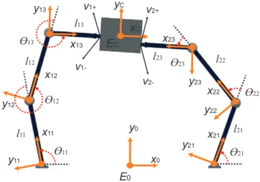
In the robotics area, many tasks are difficult or even im-possible to be performed by using a single robot. Typ-ical examples include: positioning of heavy payloads, complex assembly of multiple parts or manipulation of flexible objects. These tasks become feasible with the employment of more than one robot operating cooper-atively (Caccavale and Uchiyama, 2008). The mecha-nism presented in Figure 3 is constituted by a closed kinematic chain, where all joints are active, and con-siders a continuous contact of the end-effector with the manipulated object.
In general, cooperating robots correspond to over-actuated systems or redundant systems, where the ef-fective degrees of freedom are higher than those strictly required to perform a given task (ne> nt). This capac-ity increases the dextercapac-ity of the mechanism, and can be used to avoid joint limits, singularities and workspace obstacles, as well as to minimize the energy consump-tion and joint torques or to optimize a performance in-dex (e.g.,manipulability).
4.1
Forward kinematics
The forward kinematics map for a redundant robotic system composed by two cooperating robots can be de-scribed by means of the posture of the frame attached to the manipulated object E¯c with respect to the base frameE0¯ , determined for each manipulator that belongs to the robotic system. The structure equations of the redundant mechanism illustrated in Figure 3 are given respectively by
pc =p01+p1c | {z } robot 1
= p02+p2c | {z } robot 2
, (47)
ϕc =ϕ01+ϕ1c
| {z }
robot 1
= ϕ02+ϕ2c
| {z }
robot 2
, (48)
where
p0i∈R3: is the position vector of the end-effector frame of thei-thmanipulatorE¯iwith respect to the base frame
¯ E0.
pic∈R3: is the position vector of the manipulated ob-ject frame E¯c with respect to the end-effector frame of thei-thmanipulatorE¯i.
x
0E
0y
21!
11E
Cx
21x
22x
23x
13x
12x
11y
0y
22y
23y
13y
12y
11y
Cx
C!
12!
13!
23!
22!
21l
11l
12l
13l
23l
22
l
21v
1+v
2+
v
1-v
2-Figure 3: Cooperating robot arms carrying a rigid object.
ϕic∈R3: denotes the orientation of the manipulated object frame E¯c with respect to the end-effector frame of thei-thmanipulatorE¯i.
The structure equations introduce kinematic constraints on the system, due to the continuous contact of the robots with the manipulated object. In contrast with parallel mechanism, the number of constraints is not equal to the number of passive joints of the robots. Indeed, for the mechanism presented in Figure 3, the passive joints are associated to the contact points be-tween the manipulators and the object (Caccavale and Uchiyama, 2008).
4.2
Differential kinematics
Considering the open chain, the end-effector velocityvi+
of the i-thmanipulator is related with the velocities of the jointsθi by
v+i =Ji(θi) ˙θi, (49) where Ji is the Jacobian of the i-th manipulator, ob-tained as a function of the joint anglesθi.
Now, we considervc the velocity of the frame E¯c fixed on the manipulated object. The object velocity vi− at the contact points is related withvc by means of
v−i =Aivc, Ai = [
I −pic×
0 I
]
, (50)
whereAiis the adjoint transformation which relates the velocities of the object frame E¯c and the end-effector frame of thei-thmanipulatorE¯Ei.
The relative velocity of the each contact point can be parameterized by a velocity vectorwi by using:
v−i =v+i +HiTwi, (51) where the columns of the matrixHT
i represent the di-rections for free motion at the contact points.
The Jacobian can be rewritten in a more conventional way stacking the Jacobians for each open kinematic
chain as [
J1 0 0 J2
]
| {z }
J
˙ θ=
[
v1+ v2+
]
| {z } v+
, (52)
or equivalently
Jθ˙=v+. (53) Thus, the differential kinematics relations can be rewrit-ten as
v++HTw=v−, v−=A vc, (54) wherew= [wT
1 w2T]T, H= [H1T H2T]T andAT= [AT1 AT2]
has full rank.
The definitionθ˙p=wand θ˙a = ˙θ allow us to represent the system in a more generally form, according to (5) and (6), by means of (Wen and Wilfinger, 1999)
˜
A[ J HT ]
| {z }
Jc
[ ˙
θa
˙ θp
]
= 0, (55)
A†[ J HT ]
| {z }
Jm
[ ˙
θa
˙ θp
]
= vc , (56)
where Ae is the annihilating matrix such that, e
that A†A=I. A possible choice forA˜ and A† is given byAe= [A2 −A1] andA†= [A−1
1 0].
Note that, from (8) and by usingJc andJm, the differ-ential kinematics equation of the object is given byvc=
¯
Jθ˙a, whereJ¯∈R3×6is given byJ¯=J
ma−JmpJcp−1Jca.
4.3
Selection matrices
The kinematic constraints of the robotic system due to the contact points are properly represented by means of a selection matrixH. This matrix acts as a filter that accepts or rejects components of motion at the contact point.
Considering the example presented in Figure 3, for the planar case a multiple robot system with compliant grip-pers does not allow translational and rotational motions of the manipulated object, which implies that H = 0. On the other hand, for a multiple robot system with-out grippers, contact points with friction can be con-sidered. In this case, only angular motions between the end-effector and the object are allowed and the selection matrixH is given by
H =
00
1
. (57)
Some examples of other types of contacts and associ-ated values of the selection matrixH are presented in (Murray et al., 1994; Wen and Wilfinger, 1999).
4.4
Kinematic control
In this section, the kinematic control approach will be used again to modify the posture of the robot manipu-lators, in order to perform a planar manipulation task with the object of interest. Here, we assume that the control objective is to lead the current posture of the objectxc= [pTc ϕc]T to a desired time varying posture
xcd(t) = [pTcd(t) ϕcd(t)]T, that is,
xc→xcd(t), ec=xcd(t)−xc→0, (58) whereec is posture error of the object.
The control scheme to be designed has to command the velocity of the all active joints of the multiple robots systemθ˙a in order to achieve the control objective (58). According to the differential kinematics of the actuated mechanism vc= ¯Jθ˙a with ne=nt, the joint velocities can be obtained from the simple inversion of the Ja-cobian matrix J¯by using θ˙a= ¯J−1v, wherev denotes the Cartesian control law, which is properly designed to avoid singular configurations.
On the other hand, for a redundant mechanism such thatne> nt, the same relationship can be rewritten in a generic form as (Sciavicco and Siciliano, 2000; Chiaverini et al., 2008):
˙
θa= ¯J†v+ (I−J¯†J¯)
| {z }
P
˙
θa0, (59)
where P denotes the orthogonal projection matrix in the null space of J¯ (i.e. J¯P = 0) and θ˙a0 is a vector of arbitrary velocities of the active joints. Note that, the right side of (59) can be interpreted as a null space velocity, whose effect is to generate internal motions that reconfigure the robot structure without changing the end-effector posture.
Considering the kinematics control problem of the over-actuated mechanism (ne> nt= 1), the control signal is equivalent to the velocity of the active joints, that is,u=
˙
θa. Then, using a control law based on a proportional with feedforward action
u= ¯J†( ˙x
cd+Kcec) + (I−J¯†J¯) ¯u , (60) where ¯uis an auxiliary control signal, the posture error dynamics is governed bye˙c+Kcec= 0, whereKcis the controller gain matrix, since the right side of the (60) is projected in the null space of J¯. Hence, for a proper choice of Kc as a positive definite matrix, implies that
limt→∞ec(t) = 0.
The auxiliary control ¯ucan be also chosen in order to improve the performance of the mechanism for the task execution. A typical choice is
¯ u= ¯K
(
∂f(θa)
∂θa )T
, (61)
where K >¯ 0 is a gain factor and f(θa)is an objective function in terms of the active joint variables, that can be chosen to satisfy a specific performance index. Some typical examples are:
Manipulability:
f(θa) = √
det( ¯JJ¯T), which vanishes at a singular configuration;
Distance from obstacles:
f(θa) = min∥p(θa)−po∥,
Joint limits: θami< θai< θaMi,
f(θa) =−
1 2n
n ∑
i=1
(
θai−θ¯ai
θaMi−θami
)2 ,
where θaMi and θami denote the maximum and
min-imum joint limits respectively, and θ¯ai is the average
value between θaMi andθami.
4.5
Kinematic singularities
The posture of the manipulator, obtained as a function of the joint anglesθ, is said to be singular if the Jacobian matrixJ¯has not full rank. From (8) we can observe that when the robot is not in a singular configuration it is possible to generate velocities and accelerations with the end-effector in certain directions. In order to evaluate the linear relation (8), the singular value decomposition (SVD) method can be used to obtain the rank of the JacobianJ¯and study quasi-linear mappings (Chiaverini et al., 2008).
In this context, the SVD of the Jacobian can be repre-sented by
¯
J =UΣVT = m ∑
i=1
σiuiviT, (62)
where U ∈Rm×m is the orthogonal matrix of output singular vectors ui, V ∈Rn×n is the orthogonal matrix of the input singular vectors vi, and Σ∈diag(D,0) ∈
Rm×n is the matrix whose diagonal submatrix D ∈
Rm×m contains the singular valuesσi of the matrix J¯. Considering thatrank( ¯J) =k, we have
σ1≥σ2≥ · · · ≥σr≥σk+1=...= 0; R( ¯J) =span{u1,· · · , uk};
N( ¯J) =span{vk+1,· · ·, vn},
where R( ¯J) denotes the range space of J¯ and N( ¯J)
denotes the null space ofJ¯. Then, the following analysis in terms of the rank of matrixJ¯can be established:
full rank (k=m): (i)σi̸= 0, i= 1,· · · , m, (ii)R( ¯J)∈
Rm, (iii)N( ¯J)∈Rn−m.
rank deficient (k < m): (i) σi̸= 0, i= 1,· · · , k, (ii)
R( ¯J)∈Rk ⊂Rm, (iii)N( ¯J)∈Rn−k.
An interpretation of this analysis in terms of velocities is presented as follows (Chiaverini et al., 2008):
Feasible velocities: For each configuration of the
ma-nipulator,R( ¯J)is the set of the end-effector velocities that can be generated by all possible joint velocitiesθ˙, and are called thefeasible velocitiesof the end-effector. The base of R( ¯J) is obtained by the first k output singular vectors, which represent the independent lin-ear combinations of the single components of the end-effector velocities. Then, the effect of a singularity is to decrease the dimension of R( ¯J), by eliminating a linear combination of the components of the end-effector velocities that belong to the feasible velocities space.
Null space velocities: For each configuration of the
ma-nipulator,N( ¯J)is the set of joint velocitiesθ˙, that do not produce any end-effector velocity, and are called thenull space velocities. The base ofN( ¯J)is obtained by the lastn−kinput singular vector, which represent the independent linear combinations of the velocities at each joint. The effect of a singularity is to increase the dimension ofN( ¯J), by adding more one indepen-dent linear combination of the joint velocities, which produces a zero end-effector velocity.
5
NONHOLONOMIC ROBOTS
Other examples of robotic systems with constraints are the wheeled mobile robots and multifingered robot hands. In general, a constraint is said to be holonomic if it restricts the robot motion to a smooth hypersurface of the configuration space. Holonomic constraints can be represented locally as algebraic constraints on the robot configuration spaceci(θ) = 0fori= 1,· · · , r. On the other hand, if the allowable motions of the robotic system are restricted by the velocity constraint in the form
A(θ) ˙θ= 0,
whereA∈Rr×nrepresents a set ofrvelocity constraints that are not integrable, the constraint is said to be non-holonomic.
These constraints arise in robotic systems , where an-gular moment is conserved, as well as rolling contact is involved. Nonholonomic constraints occur when the instantaneous velocities of the robotic system are re-stricted to an n−r dimensional subspace, but the set of reachable configurations is not constrained to some
n−rdimensional hypersurface in the robot configura-tion space (Murray et al., 1994).
allowable trajectories of the system can be written as possible solutions of the control system
˙
θ= ˜A(θ)u , (63) where u∈Rn−r is the control signal to be designed in order to drive the current configuration θ ∈ Rn to a desired time-varying configurationθd(t)∈Rn.
The main difficulty arises from the fact that this sys-tem has not right pseudoinverse, sinceAcontains more rows than columns, and the linearized system is not controllable (Murray et al., 1994). However, there are different approaches to accomplish the control of this systems, that consists of both physical remove of the nonholonomic constraints and the application of ad-vanced control tools based on nonlinear control the-ory, differential geometry or optimal control (Murray et al., 1994; Bloch, 2003).
6
SIMULATION RESULTS
In this section, we present simulations results obtained from a Four-Bar linkage mechanism, a planar Gough-Stewart platform and two cooperating robot arms com-posed by four revolution joints. The adopted struc-tural dimensions are: l0= 1 m, l1= 1.2 m, l2= 1.4 m,
l3 = 0.6m, l4 = 1.4m, l = 5m, l11 = l12 = 1.2 m,
l21 =l22 = 1m and l13 =l23 = 0.6m. For the con-sidered lengths of links, we define the following limits:
θ1∈[ 0.72 2.27 ]rad and ϕ∈[ 5.88 7.89 ]rad. The con-trol parameters are: kϕ= 50rad s−1 and Ks=Kc =
diag(50mm s−1,50mm s−1,1rad s−1).
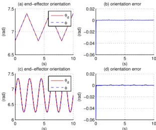
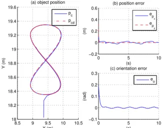
The time evolution for the orientation error of the Four-Bar linkage mechanism for train of ramps and sinusoidal references are shown in Figures 4(b) and 4(d) respec-tively. Figures 5(b) and 5(c) illustrate the time evolu-tion of the posievolu-tion error and orientaevolu-tion error for the Gough-Stewart platform. The position and orientation errors for the object handled by two cooperating robots are shown in Figures 6(b) and 6(c) respectively. The trajectory following for all mechanisms are presented re-spectively in Figures 4(a)-4(c), 5(a) and 6(a), where it can observe that a good performance is achieved by us-ing the presented methodology.
7
CONCLUSIONS AND PERSPECTIVES
This work presents a control methodology for robotic systems under kinematics constraints based on a novel scheme in the robotics literature, which regards the con-straints on passive joint velocities. The key idea is to consider the kinematic constraints of the mechanism from their structure equations, rather than explicitly
0 5 10
6.5 7 7.5
(a) end−effector orientation
(s)
(rad)
φd φ
0 5 10
−0.06 −0.04 −0.02 0 0.02
(b) orientation error
(s)
(rad)
0 5 10
6 6.5 7 7.5
(c) end−effector orientation
(s)
(rad)
0 5 10
−0.06 −0.04 −0.02 0 0.02
(d) orientation error
(s)
(rad)
φd φ
Figure 4: Four-Bar linkage mechanism: (a) end-effector orien-tation: train of ramps, (b) orientation error, (c) end-effector orientation: sinusoidal wave form, (d) orientation error.
10 12 14 16 18 10
11 12 13 14 15 16 17 18
(a) platform position
X (m)
Y (m)
p
pd
0 5 10
−1.5 −1 −0.5 0 0.5
(s)
(m)
(b) position error
ep
x
e py
0 5 10
−1.5 −1 −0.5 0 0.5
(c) orientation error
(s)
(rad)
Figure 5: Gough-Stewart platform: (a) platform position, (b) position error, (c) orientation error.
invoking the constraint equation. In order to show the applicability of the presented methodology, simulations results were included for a Four-Bar linkage mechanism, a planar Gough-Stewart platform and two cooperating robots.
8.5 9 9.5 10 10.5 18
18.2 18.4 18.6 18.8 19 19.2 19.4 19.6
(a) object position
X (m)
Y (m)
p c p
cd
0 5 10
−0.2 0 0.2 0.4 0.6
(s)
(m)
(b) position error
e px ep
y
0 5 10
−0.1 0 0.1 0.2 0.3
(s)
(rad)
(c) orientation error
e o
Figure 6: Cooperating robots: (a) object position, (b) position error, (c) orientation error.
Some research topics, applied to redundant manipula-tors and parallel robots, that can be investigated fol-lowing the ideas presented in this work are: to consider the dynamic control problem for these mechanisms, re-lax the assumption of the robot kinematics to be fully known and develop a strategy for singularity and obsta-cle avoidance.
ACKNOWLEDGMENTS
This work was partially supported by Brazilian Found-ing agencies CNPq, CAPES and FAPERJ.
REFERENCES
Bicchi, A. and Prattichizzo, D. (2000). Manipulabil-ity of cooperating robots with unactuated joints and closed-chain mechanisms, IEEE Transactions
on Robotics and Automation16(4): 336–345.
Bloch, A. M. (2003). Nonholomic Mechanics and Con-trol, Springer Verlag.
Caccavale, F. and Uchiyama, M. (2008). Cooperative manipulators,in B. Siciliano and O. Khatib (eds),
Springer Handbook of Robotics, 1st edn,
Springer-Verlag Ltd., pp. 701–718.
Caurin, G. A. P. and Pedro, L. M. (2009). Hybrid mo-tion planning approach for robot dexterous hands, Journal of the Brazilian Society of Mechanical
Sci-ences & Engineering31(4):289–296.
Cheng, H., Yiu, Y.-K. and Li, Z. (2003). Dynamics and control of redundantly actuated parallel
manipula-tors, IEEE/ASME Transactions on Mechatronics 8(4): 483–491.
Chiaverini, S., Oriolo, G. and Walker, I. D. (2008). Kinematically redundant manipulators, in B. Si-ciliano and O. Khatib (eds), Springer Handbook of
Robotics, 1st edn, Springer-Verlag Ltd., pp. 245–
268.
Freitas, G. M., Gleizer, G., Lizarralde, F., Hsu, L. and dos Reis, N. R. S. (2010). Kinematic reconfigurabil-ity control for an environmental mobile robot op-erating in the amazon rain forest,Journal of Field
Robotics27(2): 197–216.
Gosselin, C. and Angeles, J. (1990). Singularity analysis of closed-loop kinematic chains,IEEE Transactions
on Robotics and Automation6(3): 281–290.
Kim, J., Park, F. C., Ryu, S. J., Kim, J., Hwang, J. C., Park, C. and Iurascu, C. C. (2001). Design and analysis of a redundantly actuated parallel mech-anism for rapid machining, IEEE Transactions on
Robotics and Automation17(4): 423–434.
Kövecses, J., Piedbœuf, J.-C. and Lange, C. (2003). Dynamics modeling and simulation of constrained robotic systems, IEEE/ASME Transactions on
Mechatronics8(2): 165–177.
Liu, G., Lou, Y. and Li, Z. (2003). Singularities of parallel manipulators: A geometric treatment, IEEE Transactions on Robotics and Automation 19(4): 579–594.
Merlet, J.-P. (1993). Parallel manipulators: state of the art and perspectives,Advanced Robotics8(6): 589– 596.
Merlet, J.-P. and Gosselin, C. (2008). Parallel mecha-nisms and robots, in B. Siciliano and O. Khatib (eds), Springer Handbook of Robotics, 1st edn, Springer-Verlag Ltd., pp. 269–285.
Murray, R. M., Li, Z. and Sastry, S. S. (1994). A
Math-ematical Introduction to Robotic Manipulation, 1st
edn, CRC Press Inc., Boca Raton, FL, USA.
Namvar, M. and Aghili, F. (2005). Adaptive motion-force control of coordinated robots interacting with geometrically unknown environments,IEEE
Trans-actions on Robotics21(4): 678–694.
O’Brien, J. F., Jafari, F. and Wen, J. T. (2006). Determination of unstable singularities in paral-lel robots with N-arms, IEEE Transactions on
Pazelli, T., Terra, M. H. and Siqueira, A. A. (2011). Experimental investigation on adaptive robust con-troller designs applied to a free-floating space ma-nipulator,Control Engineering Practice1(1): 1–14.
Pietsch, I. T., Krefft, M., Becker, O. T., Bier, C. C. and Hesselbach, J. (2005). How to reach the dynamic limits of parallel robots ? an autonomous control approach, IEEE Transactions on Automation
Sci-ence and Engineering2(4): 369–380.
Ribeiro, L., Guenther, R. and Martins, D. (2008). Screw-based relative jacobian for manipulators co-operating in a task, ABCM Symposium Series in
Mechatronics3: 276–285.
Rosario, J. M., Dumur, D. and Machado, J. T. A. (2007). Control of a 6-DOF parallel manipulator through a mechatronic approach,Journal of
Vibra-tion and Control13(9): 1431–1446.
Sciavicco, L. and Siciliano, B. (2000). Modelling and
Control of Robot Manipulators, 2nd edn,
Springer-Verlag Ltd., New York, NY, USA.
Siciliano, B. (1990). Kinematic control of redundant robot manipulators: A tutorial, Journal of
Intelli-gent and Robotic Systems3(3): 201–212.
Siciliano, B., Sciavicco, L., Villani, L. and Oriolo, G. (2008).Robotics: Modelling, Planning and Control, 1st edn, Springer-Verlag London Ltd.
Simas, H., Guenther, R., da Cruz, D. F. M. and Mar-tins, D. (2009). A new method to solve robot in-verse kinematics using Assur virtual chains, Robot-ica 27: 1017–1022.
Tinos, R., Terra, M. H. and Ishihara, J. Y. (2006). Mo-tion and force control of cooperative robotic ma-nipulators with passive joints, IEEE Transactions
on Control System Technology14(4): 725–734.
Wen, J. T. and O’Brien, J. F. (2003). Singularities in three-legged platform-type parallel mechanisms, IEEE Transactions on Robotics and Automation 19(4): 720–727.
Wen, J. T.-Y. and Wilfinger, L. S. (1999). Kinematic manipulability of general constrained rigid multi-body systems,IEEE Transactions on Robotics and
Automation 15(3): 558–567.
Zhang, G.-F. and Gao, X.-S. (2006). Planar generalized stewart platforms and their direct kinematics, in H. Hong and D. Wang (eds),Automated Deduction
in Geometry, Vol. 3763 of Lecture Notes in
Com-puter Science, Springer-Verlag Berlin / Heidelberg,